
smallpt[1] 是一个仅有 99 行的迷你光线追踪渲染器,在极小的体积下实现了图元、材质、光源、场景、相机、采样器、积分器等模块,可以说麻雀虽小五脏俱全。关于 smallpt 是如何实现这些功能的,网络上已经有些很好的介绍[2][3][4]。
pbrt[5] 既是一个多功能光线追踪渲染器的名字,也是对应书籍的简称[6],书中以文学编程 Literate Programming 的方式,介绍了这个读者如果能看懂就看得懂,看不懂就看不懂的渲染器。pbrt 具有一个相当优秀的架构,给很多渲染器带来了启发[7][8][9]。下文中提到的 pbrt 指渲染器,PBRT 指书籍。
pbrt 工作时的主要流程,主要是在 Render() 函数里的渲染循环
smallpt 和 pbrt 虽然体量和功能差异巨大,但在笔者眼里却有着一样的核心功能:蒙特卡洛光线追踪(Monte Carlo Ray Tracing),这就像王垠说的:
很多人都不知道,有一天我用不到一百行 Scheme 代码就写出了一个「深度学习框架」,它其实是一个小的编程语言。虽然没有性能可言,没有 GPU 加速,功能也不完善,但它抓住了 PyTorch 等大型框架的本质——用这个语言写出来的函数能自动求导。这种洞察力才是最关键的东西,只要抓住了关键,细节都可以在需要的时候琢磨出来。几十行代码反复琢磨,往往能帮助你看透上百万行的项目里隐藏的秘密。
如何阅读别人的代码 https://www.yinwang.org/blog-cn/2020/02/05/how-to-read-code
通过阅读一个小规模的软件,来了解这一类型软件的架构模式是很常见的做法[10]。但 smallpt 为了控制体积实在太简略了一点,导致它的结构并没有那么清晰,想从 smallpt 里看出 pbrt 的架构并不容易,而且它那 99 行的代码里还涉及了大量的理论技术。
本文将基于 pbrt 的架构一步步改写 smallpt,通过每一步的实际代码去解释蒙特卡洛光线追踪和 pbrt 的大致架构,方便对光线追踪、全局光照感兴趣的同学了解学习。
文中对应的所有代码位于 infancy/ky,需要用最新的 C++ 编译器编译。
最后由于笔者经验水平有限,文中多有错漏,敬请各位读者批评指正。
原版的 smallpt
- 代码:smallpt.cpp
这里为了方便阅读,先加了一些空格。
参考这张经典的光线追踪示意图,先来看看 smallpt 里目前可以看懂的结构吧。
")
首先直接把那 99 行代码拷贝下来是编译不过的,缺少常量 M_PI 和函数 erand48(),这里补充了一下:
 // line 1~7
 // http://www.kevinbeason.com/smallpt
 #include "erand48.h"// pseudo-random number generator, not in <stdlib.h>
 #include <math.h>   // smallpt, a Path Tracer by Kevin Beason, 2008
 #include <stdlib.h> // Make : g++ -O3 -fopenmp smallpt.cpp -o smallpt
 #include <stdio.h>  //        Remove "-fopenmp" for g++ version < 4.2

 #define M_PI 3.141592653589793238462643
最基础的三维向量 Vector3,同时充当了位置 Point3,法线 Normal3 和颜色 Color。
注意它为了压缩 radiance(...) 函数的体积,把外积 cross() 用 operator% 来表示了。
 // line 9~20
 struct Vec {        // Usage: time ./smallpt 5000 && xv image.ppm
   double x, y, z;                  // position, also color (r,g,b)

   Vec(double x_=0, double y_=0, double z_=0){ x=x_; y=y_; z=z_; }

   Vec operator+(const Vec &b) const { return Vec(x+b.x,y+b.y,z+b.z); }
   Vec operator-(const Vec &b) const { return Vec(x-b.x,y-b.y,z-b.z); }
   Vec operator*(double b) const { return Vec(x*b,y*b,z*b); }
   Vec mult(const Vec &b) const { return Vec(x*b.x,y*b.y,z*b.z); }
   Vec& norm(){ return *this = *this * (1/sqrt(x*x+y*y+z*z)); }
   double dot(const Vec &b) const { return x*b.x+y*b.y+z*b.z; } // cross:
   Vec operator%(Vec&b){return Vec(y*b.z-z*b.y,z*b.x-x*b.z,x*b.y-y*b.x);}
 };
基于几何光学模型实现的光线类,由起点 origin o 和方向 direction d 表示,其中方向 d 一般是单位向量:
 // line 22
 struct Ray { Vec o, d; Ray(Vec o_, Vec d_) : o(o_), d(d_) {} };
材质枚举,用于区分不同物体表面外观的材质类型, 其中包含了漫反射 diffuse reflection,镜面反射 specular reflection 和菲涅尔镜面散射 fresnel specular scattering 三种类型:
 // line 24
 enum Refl_t { DIFF, SPEC, REFR };  // material types, used in radiance()
唯一的几何形状:球体,除了半径 radius rad 和位置 position p 外,还记录了表面自发光的亮度 emission e,材质类型 c 和表面反照率 albedo c(也就是日常生活中说的物体表面的颜色)。
- 当亮度
e大于 0 时,这个球体会向场景中发射亮度,照亮场景。 - 当反照率
c为 0 时,这个球体会吸收所有入射光,看起来就是黑色的。
还有一个和光线求交点的成员函数,放到下一节讲。
 // line 26~39
 struct Sphere {
   double rad;       // radius
   Vec p, e, c;      // position, emission, color
   Refl_t refl;      // reflection type (DIFFuse, SPECular, REFRactive)

   Sphere(double rad_, Vec p_, Vec e_, Vec c_, Refl_t refl_):
     rad(rad_), p(p_), e(e_), c(c_), refl(refl_) {}

   double intersect(const Ray &r) const { // returns distance, 0 if nohit
     Vec op = p-r.o; // Solve t^2*d.d + 2*t*(o-p).d + (o-p).(o-p)-R^2 = 0
     double t, eps=1e-4, b=op.dot(r.d), det=b*b-op.dot(op)+rad*rad;
     if (det<0) return 0; else det=sqrt(det);
     return (t=b-det)>eps ? t : ((t=b+det)>eps ? t : 0);
   }
 };
9 个球体,描述了整个场景。
和渲染图的场景内容比起来,前 6 个球体非常大,以至于它们的局部看起来像是平坦的,作者用它们围成了一个封闭的盒子。
接着是我们看到的镜面球体和玻璃球体,以及一个相对大一些的球形光源。
 // line 41~51
 Sphere spheres[] = {//Scene: radius, position, emission, color, material
   Sphere(1e5, Vec( 1e5+1,40.8,81.6), Vec(),Vec(.75,.25,.25),DIFF),//Left
   Sphere(1e5, Vec(-1e5+99,40.8,81.6),Vec(),Vec(.25,.25,.75),DIFF),//Rght
   Sphere(1e5, Vec(50,40.8, 1e5),     Vec(),Vec(.75,.75,.75),DIFF),//Back
   Sphere(1e5, Vec(50,40.8,-1e5+170), Vec(),Vec(),           DIFF),//Frnt
   Sphere(1e5, Vec(50, 1e5, 81.6),    Vec(),Vec(.75,.75,.75),DIFF),//Botm
   Sphere(1e5, Vec(50,-1e5+81.6,81.6),Vec(),Vec(.75,.75,.75),DIFF),//Top
   Sphere(16.5,Vec(27,16.5,47),       Vec(),Vec(1,1,1)*.999, SPEC),//Mirr
   Sphere(16.5,Vec(73,16.5,78),       Vec(),Vec(1,1,1)*.999, REFR),//Glas
   Sphere(600, Vec(50,681.6-.27,81.6),Vec(12,12,12),  Vec(), DIFF) //Lite
 };
两个用来保存图像的辅助函数,其中 toInt 还做了伽马编码(Gamma Encoding),将线性空间计算出来的颜色保存到 sRGB 空间:
 // line 53~54
 inline double clamp(double x){ return x<0 ? 0 : x>1 ? 1 : x; }
 inline int toInt(double x){ return int(pow(clamp(x),1/2.2)*255+.5); }
场景求交函数,它会遍历所有球体,找到入射光线在场景中的最近交点,其中参数 t 记录了光线到最近交点的距离,默认为一个非常大的值。
因为整个场景是封闭的,光线不会离开场景,一定可以找到交点。
 // line 56~60
 inline bool intersect(const Ray &r, double &t, int &id){
   double n=sizeof(spheres)/sizeof(Sphere), d, inf=t=1e20;
   for(int i=int(n);i--;) if((d=spheres[i].intersect(r))&&d<t){t=d;id=i;}
   return t<inf;
 }
亮度函数,对于传入的光线,先找到它与场景的最近交点,再计算交点沿光线方向发射的亮度:
 // line 62~67
 Vec radiance(const Ray &r, int depth, unsigned short *Xi){
   double t;                               // distance to intersection
   int id=0;                               // id of intersected object
   if (!intersect(r, t, id)) return Vec(); // if miss, return black

   const Sphere &obj = spheres[id];        // the hit object
其中具体的逻辑目前看起来就像一团乱码,先跳过。
// line 68~95
// ...
主函数,开头给出了图片的长宽 w 和 h,每个像素的采样数量 samps, 用光线 cam 记录相机的位置和朝向等:
 // line 97~100
 int main(int argc, char *argv[]){
   int w=1024, h=768, samps = argc==2 ? atoi(argv[1])/4 : 1; // # samples
   Ray cam(Vec(50,52,295.6), Vec(0,-0.042612,-1).norm()); // cam pos, dir
   Vec cx=Vec(w*.5135/h), cy=(cx%cam.d).norm()*.5135, r, *c=new Vec[w*h];
遍历图像平面,对每个像素向场景中投射若干光线,计算该像素的颜色。
5 个 for 循环着实有点多,这里也先跳过。
 // line 102~120
 #pragma omp parallel for schedule(dynamic, 1) private(r)       // OpenMP
   for (int y=0; y<h; y++){                       // Loop over image rows
     fprintf(stderr,"\rRendering (%d spp) %5.2f%%",samps*4,100.*y/(h-1));
     for (unsigned short x=0, Xi[3]={0,0,y*y*y}; x<w; x++)   // Loop cols

       for (int sy=0, i=(h-y-1)*w+x; sy<2; sy++)     // 2x2 subpixel rows
         for (int sx=0; sx<2; sx++, r=Vec()){        // 2x2 subpixel cols

           for (int s=0; s<samps; s++){
             double r1=2*erand48(Xi), dx=r1<1 ? sqrt(r1)-1: 1-sqrt(2-r1);
             double r2=2*erand48(Xi), dy=r2<1 ? sqrt(r2)-1: 1-sqrt(2-r2);
             Vec d = cx*( ( (sx+.5 + dx)/2 + x)/w - .5) +
                     cy*( ( (sy+.5 + dy)/2 + y)/h - .5) + cam.d;

             r = r + radiance(Ray(cam.o+d*140,d.norm()),0,Xi)*(1./samps);
           } // Camera rays are pushed ^^^^^ forward to start in interior

           c[i] = c[i] + Vec(clamp(r.x),clamp(r.y),clamp(r.z))*.25;
         }
   }
最后用 ppm[11] 格式保存图片:
 // line 122~125
   FILE *f = fopen("image.ppm", "w");         // Write image to PPM file.
   fprintf(f, "P3\n%d %d\n%d\n", w, h, 255);

   for (int i=0; i<w*h; i++)
     fprintf(f,"%d %d %d ", toInt(c[i].x), toInt(c[i].y), toInt(c[i].z));
 }
为了尽可能的压缩体积,smallpt 中没有定义显式的光源 light,材质 material,相机 camera 等结构,但对应功能都是有的。同时还用了很简略的变量名和紧凑的代码格式。
这里先添加 smallpt_format.cpp 文件,用来对原版代码做格式化,然后在 smallpt_format.cpp 的基础上添加了 smallpt_comment.cpp 文件,其中重命名了变量和函数的名字,方便下一步理解代码。
理解 smallpt
这一步首先修改了变量名和函数名,让 smallpt 的代码变得更具有可读性。然后将从实际执行流程来理解 smallpt 和蒙特卡洛光线追踪,这样的话在下一节“改写 smallpt”中我们只需要关注整体结构即可。
主函数
注释后的主函数如下:
// line 280~290
int main(int argc, char* argv[])
{
    int width = 1024, height = 768;
    int samplesPerPixel = argc == 2 ? atoi(argv[1]) / 4 : 10;

    // right hand
    Ray camera(Vector3(50, 52, 295.6), Vector3(0, -0.042612, -1).Normalize()); // camera posotion, direction
    Vector3 cx = Vector3(width * .5135 / height); // left
    Vector3 cy = (cx.Cross(camera.direction)).Normalize() * .5135; // up

    Color* film = new Vector3[width * height];
接着是生成图像的简化逻辑:

- 用两个 for 循环遍历图像平面的所有像素,再用采样器围绕每个像素生成图像平面的采样点;
- 根据采样点的位置,用相机生成光线并投射到场景中,找到最近交点;
- 计算交点沿光线发射的亮度(用颜色来表示);
- 对该像素中所有采样点的颜色取平均值,然后写入到图片中:
    // line 292 324
    #pragma omp parallel for schedule(dynamic, 1) // OpenMP
    for (int y = 0; y < height; y++) // Loop over image rows
    {
        unsigned short sampler[3] = { 0, 0, y * y * y };
        for (unsigned short x = 0; x < width; x++) // Loop cols
        {
            Color Li{};
            int i = (height - y - 1) * width + x;
            // ...
                    for (int s = 0; s < samplesPerPixel; s++)
                    {
                        // ...
                        Vector3 direction =
                            cx * (((sx + .5 + dx) / 2 + x) /  width - .5) +
                            cy * (((sy + .5 + dy) / 2 + y) / height - .5) + camera.direction;

                        Li = Li + Radiance(Ray(camera.origin + direction * 140, direction.Normalize()), 0, sampler) * (1. / samplesPerPixel);
                    } // Camera rays are pushed ^^^^^ forward to start in interior

                    film[i] = film[i] + Vector3(Clamp(Li.x), Clamp(Li.y), Clamp(Li.z)) * .25;
                }
            }
        }
    }

    // ...
其中 #pragma omp parallel for 指令可以便捷的开启 OpenMP[12] 的多线程加速功能。
这里并不打算详细介绍相机和采样器的逻辑,它们在重写后的代码里(smallpt_rewrite.cpp)会更好理解。
紧接着来看 Radiance 函数。
Radiance(...) #1
对 Radiance(...) 函数的分析会拆成几节,这里先理解下面的代码:
// line 165~173
Color Radiance(const Ray& ray, int depth, unsigned short* sampler)
{
    double distance; // distance to intersection
    int id = 0; // id of intersected object

    if (!Intersect(ray, distance, id))
        return Color(); // if miss, return black

    const Sphere& obj = Scene[id]; // the hit object
Radiance 函数首先接收入射光线并查找它与场景中的交点(因为它是是一个递归函数,所以光线不一定只来源于图像平面),在处理异常情况后,开始计算着色相关的信息。
其中场景求交函数 Intersect(...) 如下:
// line 145~163
inline bool Intersect(const Ray& ray, double& minDistance, int& id)
{
    double infinity = 1e20;
    minDistance = infinity;

    int sphereNum = sizeof(Scene) / sizeof(Sphere);
    double distance{};

    for (int i = sphereNum; i--;)
    {
        if ((distance = Scene[i].Intersect(ray)) && distance < minDistance)
        {
            minDistance = distance;
            id = i;
        }
    }

    return minDistance < infinity;
}
这里需要判断和更新光线到场景交点的最小距离。
光线求交
接着是求解光线和圆球交点的逻辑,先再次介绍一下光线:
using UnitVector3 = Vector3;

// line 46~52
struct Ray
{
    Point3 origin;
    UnitVector3 direction;

    Ray(Point3 origin_, UnitVector3 direction_): origin(origin_), direction(direction_) {}
};
其中 UnitVector3 只是一个提示,没有实际的约束作用。
光线可以被定义为三维空间中的一条射线:
其中 起点 $\mathrm{O}$, 方向 $\mathrm{D}$ 已知
- 代入距离 $t$ 可以得到一个新的端点 $\mathrm{R}(t)$
- 将 $\mathrm{R}(t)$ 视作一个已知点, 代入某个方程中, 则可以得到距离 $t$

然后是球体的定义:
其中 $P$ 是球上任意一点 $\left(x_{p}, y_{p}, z_{p}\right)$,$C$ 是球的圆心 $\left(x_{c}, y_{c}, z_{c}\right)$,$r$ 是球的半径。

当光线和球体相交时,意味着光线的另一端点在球面上:
为了简化形式,将其中的 $\mathrm{O}-\mathrm{C}$ 记作新的向量 $\mathrm{CO}$,就有
根据球体的定义继续推导:
其中所有的向量都会做点积变成标量,并且只有一个未知数 $t$,这样就得到了一元二次方程:
其中
方程的解为
最后一步为了省去负号,将 $\mathrm{OC}$ 掉转方向为 $\mathrm{CO}$。
下面是球体 Sphere 的求交函数,首先判断方程是否有解:
// line 103~110
struct Sphere
{
    double radius;
    Point3 center;

    double Intersect(const Ray& ray) const
    {
        Vector3 oc = center - ray.origin;
        double neg_b = oc.Dot(ray.direction);
        double det = neg_b * neg_b - oc.Dot(oc) + radius * radius;

        if (det < 0)
            return 0;
        else
            det = sqrt(det);
然后分情况去找最近的非负交点:
蓝色点代表光线的起点,红色点代表交点
        // line 112~123
        double epsilon = 1e-4;
        if (double t = neg_b - det; t > epsilon)
        {
            return t;
        }
        else if (t = neg_b + det; t > epsilon)
        {
            return t;
        }

        return 0;
    }
};
其中 epsilon 是为了避免浮点精度带来的误差。
表面着色
在得到光线和场景最近的交点后,就可以计算交点沿光线方向发射的亮度 $L_{\mathrm{o}}\left(\mathrm{p}, \omega_{\mathrm{o}}\right)$,简单来说就是这个交点会显示什么颜色,也就是所谓的着色 Shading ,此时我们的注意力就可以从具体的几何形状转移到单个交点上了。更进一步的,可以去计算交点的切线空间,将所有着色计算都放到这个切线空间里完成。

不过 smallpt 的着色计算是在世界空间里完成的。
在得到了距离 $t$ 以后,首先需要计算所有的着色信息,首先包括交点的位置 $\mathrm{p}$、法线 $\mathrm{n}$ 和表面反照率 “$f_r$”:
关于表面反照率 “$f_r$”
Color Radiance(const Ray& ray, int depth, unsigned short* sampler)
{
    double distance; // distance to intersection
    int id = 0; // id of intersected object

    if (!Intersect(ray, distance, id))
        return Color(); // if miss, return black

    const Sphere& obj = Scene[id]; // the hit object

    //...

    // line 179~182
    // intersection property
    Vector3 position = ray.origin + ray.direction * distance;
    Normal3 normal = (position - obj.center).Normalize();

    Color f = obj.color; // bsdf value
    // ...
接着是交点 $\mathrm{p}$ 朝相机的方向 $\omega_{\mathrm{o}}$,这其实就是入射光线的反方向 -ray.direction。而交点朝光源的方向 $\omega_{\mathrm{i}}$ 可以由 $\mathrm{p}_{\text{light}} - \mathrm{p}$ 得到,最后需要的信息是光源向交点发出的亮度 $L_{\mathrm{emit}}\left(\mathrm{p}, \omega_{\mathrm{i}}\right)$。
于是单个点光源经过交点 $\mathrm{p}$ 朝相机方向 $\omega_{\mathrm{o}}$ 发出的反射光为*:

其中
- 沿入射光线进入相机的亮度用 $L_{\mathrm{i}}\left(\mathrm{p}_\text{camera}, -\omega_{\mathrm{o}}\right)$ 表示,它等于交点 $\mathrm{p}$ 朝 $\omega_{\mathrm{o}}$ 方向发射的亮度 $L_{\mathrm{o}}\left(\mathrm{p}, \omega_{\mathrm{o}}\right)$,所以下文就暂时省略掉 $L_{\mathrm{i}}\left(\mathrm{p}_\text{camera}, -\omega_{\mathrm{o}}\right)$ 。
- 交点 $\mathrm{p}$ 沿 $\omega_{\mathrm{i}}$ 方向接收到的亮度用 $L_{\mathrm{emit}}(\mathrm{p}, \omega_{\mathrm{i}})$ 表示,这也是点光源朝这个方向发射(emit)的亮度。
- 对于接收到的亮度 $L_{\mathrm{emit}}(\mathrm{p}, \omega_{\mathrm{i}})$ ,表面交点会吸收一部分,反射一部分(通过表面反照率 $\rho$ 决定反射多少亮度),那么被反射的亮度 $\rho L_{\mathrm{emit}}(\mathrm{p}, \omega_{\mathrm{i}})$ 里,有多少会被反射到 $\omega_{\mathrm{o}}$ 方向上呢,或者说反射亮度 $\rho L_{\mathrm{emit}}(\mathrm{p}, \omega_{\mathrm{i}})$ 在交点 $\mathrm{p}$ 的半球方向上是怎么分布的?这个比例的大小由函数 $f_{r}\left(\mathrm{p}, \omega_{\mathrm{o}}, \omega_{\mathrm{i}}\right) $ 来决定,它就是著名的 双向反射分布函数 BRDF(Bidirectional Reflectance Distribution Function)。
根据现实物体表面外观特征总结出的三个常用 BRDF, 依次是 
完全漫反射分布: 反射亮度在半球所有方向上均匀分布
光泽镜面反射分布:围绕着反射方向分布
完全镜面反射分布:只在反射方向上分布
对于完全漫反射 BRDF 更形象的可视化
- 最后是末尾的余弦项 $\cos \theta_{\mathrm{i}}$,这一项非常重要,但完整介绍它需要更多的前置知识,这里只举个例子:假如下面的这个光源处在接近地平线的方向上,也就是 $\theta \approx 90\degree$ 时,交点还能接收到和原来一样多的亮度吗?
朗伯余弦定律 Lambert’s Law
而当场景中有多个点光源时,可以通过求和来计算反射光:

这就是着色时常用的计算方式了。
然后来看看 smallpt 的光源:

一个球形光源,或者说是一个面积光源。这是全新的情况🙄。
从光线追踪的理论算法和代码实现来看,它一直都在处理各种点:图像平面的采样点,几何物体上的交点,点状的光源——光线追踪是一类基于点采样的算法,现在碰到了面积光源,还管用吗?
不妨先来观察一下,一开始在图像平面渲染物体的情况,为什么发射一根根光线就能把物体给完整渲染出来呢?因为这些光线对应着物体上的大量交点:
对于面积光源,能不能把着色交点当作是一个新的相机,向光源上发射大量的光线?感觉可以一试。

但具体要发射多少光线,怎么确定光线的方向,把返回的亮度全部累加起来就好了吗……这个做法会带来一连串新的问题,不过它又和已经处理过的情况类似:这不就是计算多个点光源嘛。
换句话说,能不能用计算多个点光源的方式来计算面光源?在回答这个问题之前,需要先做一些铺垫。
*彩蛋:smallpt 的漫反射计算
看看原版代码,smallpt 也是把面光源当点光源算的吧:
   // line74~81
   if (obj.refl == DIFF){                  // Ideal DIFFUSE reflection
     // ...
     return obj.e + f.mult(radiance(Ray(x,d),depth,Xi));

   } else if (obj.refl == SPEC)            // Ideal SPECULAR reflection
     return obj.e + f.mult(radiance(Ray(x,r.d-n*2*n.dot(r.d)),depth,Xi));
   // ...
看起来和计算点光源的方式差不多,对于表面漫反射的情况竟然只发射一根光线,而且还把余弦项给漏掉了🤣。
事实真的如此吗?还请继续往下看。
蒙特卡洛方法
很多问题在数学上都可以归结为一个方程(组),它代表了对问题的抽象和泛化,将复杂的问题变简单,特殊的问题变一般——然而很多方程又没有解析解。
当我们无法求得方程的精确结果,或者只需要一个大概结果时,数值方法 Numerical Method 就登场了,它通过插值、逼近、拟合等多种手段去近似问题的解,下面用一个例子来介绍。
圆周率 $\pi$ 是多少
这个大家都知道近似值,但假如要自己动手算呢?
有一种用几何面积去计算的办法:假如现在有一个边长为 $2r$ 的正方形,里面放置一个半径为 $r$ 的圆形:

可以得到:
于是这就成了一个先有 $\pi$ 还是先有面积的问题。
假如在这个正方形中随机投入大量采样点,那么大部分采样点应该会落入圆形中,并且圆形内的点占所有点的比例,应该和两者的面积成正比,也就是
于是就有
这样就将求面积的确定性结果转化为了一个随机性的估计值。虽然每一次估计的结果都会不一样,但因为每个采样点都是随机分布的,估计的结果总体上会围绕着真实结果分布(比真实结果大一些或小一些)。并且随着投入的采样点越多, 这个估计值也会越精确。
最重要的是,这种方法非常简单直观,可以很容易用计算机去模拟:
from random import random

square = 10000
circle = 0

for i in range(1, square):
    x, y = random(), random();
    if (x**2 + y**2) <= 1.0:
        circle += 1

pi = 4 * (circle/square)

print('%s' % pi)
上面这种通过大量随机样本进行模拟的方法,就被称为蒙特卡罗方法 Monte Carlo method [13][14],它是一种常见的数值方法。
类似的,我们还可以用这种估算面积的方法来求积分

通过
可以得到
然而实际操作起来,会发现它的效率非常低[14],要用大量的样本才能趋近于真实值。
更好的估算积分
对于函数 $f(x)$ 在区间 $[a, b]$ 积分值
如果把 $I$ 看作是一块面积的话,也可以把它写成
其中 $\bar{f(x)}$ 是$f(x)$ 在区间 $[a, b]$ 上的平均值。

对于一个没有解析解的积分,如果我们能迅速的估算出这个 $\bar{f(x)}$,就可以计算积分的近似值。
对于均值 $\bar{f(x)}$,有
当然,这也可以根据平均值的定义直观得到:
这里显然是无法去计算无穷多个 $ f\left(x\right) $ 的,那就等同于求积分值了。但既然说过只是去估算,那就好办了:
可以仿照在面积上随机采样的做法,在这个积分的定义域 $[a, b]$ 上随机投入大量的采样点 $X_{i}$,计算每个 $X_{i}$ 的函数值 $f(X_{i})$, 用所有函数值 $f(X_{i})$ 的均值去估算 $\bar{f(x)}$:
在区间 $[a, b]$ 中随机采样若干个 $X_{i}$ 
那么就有
这样我们就从直接在(二维)面积上采样,降低成了在积分的(一维)定义域上采样。
为了方面接下来的叙述,这里把均值 $\bar{f(x)}$ 的近似估计记作 $\hat{f(x)}$:
需要注意的是 $ \hat{f(x)} $ 并不是一个值,而是一个未知量,因为在做估计之前它的大小是不确定的。只有等到实际去做估计时,根据随机采样点的数量和分布情况计算出 $ \hat{f(x)} $ 。因此称 $ \hat{f(x)} $ 为均值 $ \bar{f(x)}$ 的估计量 estimator,它是由一组随机样本点 $X_{1}, X_{2} \cdots X_{N}$ 决定的变化量。
这里同样把积分 $I$ 的估计量记作 $\hat{I}$:
(有的书中把 $ \hat{f(x)} $ 记为 $ f(x)_{N}$,$ \hat{I} $ 记为 $ I_{N}$)
那么这有什么用呢?
首先在使用面积之比估算积分时,要先找到一个能将整个积分区域包裹在内的区域,当积分区域不规则时,积分面积占总面积的比值较小,估计结果的准确性就会非常低:
假如左边在面积上采样,右边在定义域上采样,那么使用相同数量的采样下,右边显然能更高效的使用采样点
有兴趣的同学可以尝试在三维空间中,根据球体和正方体的体积之比来估算圆周率 $\pi$,会发现使用相同数量的样本下,准确性进一步降低了。
而这种新的估算方法是在积分的定义域上进行采样,而很多目标积分的定义域往往是规则的,非常方便做采样,也更能有效的利用采样点。
更重要的是,这让我们可以很容易将其应用到具有不同维度,不同形式的积分上。
例如对于二维积分
只需要在对应的区间 $[x_{0},x_{1}] \times [y_{0},y_{1}]$ 上随机投入采样点 $X_{i}$ 就好了,对应的估计量是:
比如说估算这个半球的体积
又比如要估算半球上某个立体角 $\Omega$ 的球面度,这可以通过对单位立体角做积分来获得:
本文中的 $\Omega$ 一般代表半球方向的集合
平面角的定义是圆周上弧长对半径的比值 $\theta = l / r $,单位是弧度
立体角是平面角在三维空间中的推广,
它的定义是球面上面积对半径平方的比值:$\Omega = A / r^{2}$,单位是球面度
要在一个球面上做积分,听起来很棘手的样子,但根据立体角的定义,可以将它转化成一个面积积分,看着就比较直观了:
还可以在此基础上,将面积转化为球面坐标 $(\theta, \phi)$ 来表示:

那么就只需要在半球的垂直方向上随机采样,对应的估计量是:
可以用上面两种做法去计算其它类型的立体角积分。
以上这些使用大量样本去估算积分的方法,被称为蒙特卡洛积分 Monte Carlo Integral。
估算光照
当场景中出现面积光源时,可以将面积光源对交点 $\mathrm{p}$ 所围的成立体角记作 $\Omega$,用这个立体角的积分来计算反射光:
但实际上我们无法直接求解这个积分,它没有解析解(根据物体表面材质的属性,$f_{r}\left(\mathrm{p}, \omega_{\mathrm{o}}, \omega_{\mathrm{i}}\right) $ 可能会非常复杂)。
但前面已经提到过,光线追踪是一种点采样技术,至少还可以在这个面积光源上进行点采样,计算单个方向上的反射光。
积分没有解析解,但可以在定义域上采样若干个样本……(蒙特卡洛积分:谁在叫我?)
那废话不多说,开始估算吧:
实际代码中,会在面积光源的表面上采样位置,连接它与交点生成方向 $\omega_{\mathrm{i}}$,而不是在立体角 $\Omega$ 中采样方向。这里为了方便先这么表示。
进一步的,我们可以将交点上半球方向的所有入射光 $L_{\mathrm{input}}$(包括光源发射的光 $L_{\text{emit}}$ 和其它点反射的光 $L_{\text{reflection}}$),统一用一个半球积分来表示:
这就是著名的反射率方程 Reflectance Equation,它描述了物体表面交点 $\mathrm{p}$ 会将半球方向上接收到的所有光照,反射多少到观察方向 $ \omega_{\mathrm{o}}$ 上。为了计算方便,其中发射光方向 $ \omega_{\mathrm{o}}$ 和入射光方向 $ \omega_{\mathrm{i}}$ 都是远离交点 $\mathrm{p}$ 的。
对于这个方程,可以想象在晴天的户外散步时,眼前的某个物体会在其表面半球的所有方向上接收到光照
考虑到交点本身也可能会发光(比如它处在一个面积光源上),把这部分也加上去:
它表达的是:
- 为了求出某个像素的颜色,可以用相机 $\mathrm{p}_\text{camera}$ 向场景中投射光线 $Ray \left(\mathrm{p}_\text{camera}, -\omega_{\mathrm{o}}\right)$, 计算沿这条相机光线返回的亮度 $L_{\mathrm{input}}\left(\mathrm{p}_\text{camera}, -\omega_{\mathrm{o}}\right)$;
- 为了计算 $L_{\mathrm{input}}\left(\mathrm{p}_\text{camera}, \omega_{\mathrm{o}}\right)$ ,可以先找到相机光线在场景中的交点 $\mathrm{p}$,计算交点朝方向 $\omega_{\mathrm{o}}$ 发出的亮度 $L_{\mathrm{output}}\left(\mathrm{p}, \omega_{\mathrm{o}}\right) $,它就是相机光线要返回的亮度 $L_{\mathrm{input}}\left(\mathrm{p}_\text{camera}, -\omega_{\mathrm{o}}\right)$;
- 但是为了计算交点发出的亮度 $L_{\mathrm{output}}\left(\mathrm{p}, \omega_{\mathrm{o}}\right) $,需要先求出交点在半球所有方向上接收到的亮度 $L_{\mathrm{input}}\left(\mathrm{p}, \omega_{\mathrm{i}}\right)$;
- 接着为了求出交点某个方向上接收到的亮度 $L_{\mathrm{input}}\left(\mathrm{p}, \omega_{\mathrm{i}}\right)$,可以再次发射光线,找到对应的场景交点,这就和计算相机接收到的 $L_{\mathrm{input}}\left(\mathrm{p}_\text{camera}, \omega_{\mathrm{o}}\right)$ 一样——整个过程是递归的,也就是只要能(递归的)求解出 $L_{\mathrm{input}}\left(\mathrm{p}, \omega_{\mathrm{i}}\right)$,就能计算场景中的所有光照!
- 动态演示
smallpt 通过递归求解这个方程,实际运行过程和图中的光线方向相反
这就是著名的渲染方程 Rendering Equation,它完整描述了交点 $\mathrm{p}$ 朝 $ \omega_{\mathrm{o}}$ 方向反射的亮度是多少,代表了对渲染图像这个问题的抽象和泛化,现实中所有几何光学现象(反射,折射,阴影,焦散……)都可以被统一到这个方程里,或者说根据渲染方程可以得到全局光照 Global illumination 的效果。
为了方便看清楚渲染方程的全貌,这里把 $L_{\mathrm{input}}\left(\mathrm{p}_\text{camera}, \omega_{\mathrm{o}}\right)$ 也加上了,可以看出来它是一个递归方程,smallpt 的 randiance(...) 函数求解的就是单个 $L_{\mathrm{input}}\left(\mathrm{p}, \omega_{\mathrm{i}}\right)$ 的大小。
而对它的估算也是一样的,只是这次不是采样单个光源,而是所有的入射光 $L_{\mathrm{input}}\left(\mathrm{p}, \omega_{\mathrm{i}}\right)$ ,所以我们直接对整个半球方向进行采样:

实际代码中,每次往往只会在半球方向中采样一根光线(具体原因要等到展开渲染方程的时候再解释),这样就有
大功告成,这样不仅解决了单个面积光源的计算,全局光照的效果也近在眼前了!
来看看 smallpt 的代码:
    // line 194~212
    if (obj.materialType == MaterialType::Diffuse) { // Ideal DIFFUSE reflection
        double random1 = 2 * Pi * erand48(sampler);
        double random2 = erand48(sampler);
        double random2Sqrt = sqrt(random2);

        // shading coordinate on intersection
        Vector3 w = normal;
        Vector3 u = ((fabs(w.x) > .1 ? Vector3(0, 1, 0) : Vector3(1, 0, 0)).Cross(w)).Normalize();
        Vector3 v = w.Cross(u);

        // Cosine importance sampling of the hemisphere for diffuse reflection
        Vector3 wi_direction = (u * cos(random1) * random2Sqrt + v * sin(random1) * random2Sqrt + w * sqrt(1 - random2)).Normalize();

        return obj.emission + f * radiance(Ray(position, wi_direction), depth, sampler);
    }
这段代码的意思是:
看起来对不上的样子(早就说过了,smallpt 算的是点光源,还给算错了😑)...... 等等,这段注释 // Cosine importance sampling of the hemisphere for diffuse reflection 是什么意思?
材质特性

要解释这行注释,还得先从物体的表面外观说起。上文已经说过了,对于日常生活中常见的表面外观,可以抽象成下面三种模型:
它们描述了入射光中被反射的部分,在交点半球方向上的分布情况,这种反射的分布被表达为不同的 BRDF 函数。
完全镜面反射 Ideal Specular Reflection
当物体表面具有这种特征时,反射光只会分布在镜面反射的方向上,其它方向都为 0,也就是
这可以将 $f_{\mathrm{r}}\left(\mathrm{p}, \omega_{\mathrm{o}}, \omega_{\mathrm{i}}\right)$ 作为 单位脉冲函数(Dirac delta function) 的复合函数来表示:
其中
函数中的分母只是为了抵消下面的余弦项:
这个时候再做积分就没有意义了,更不需要用蒙特卡洛积分,因为在半球上随机采样方向时,根本就不可能采样到反射方向,估算的结果将始终为 0。
光泽反射 Glossy Reflection
对于光泽表面的情况,可以看到大部分光线都围绕在反射方向上,或者说假如有若干条光线击中点 $\mathrm{p}$ 后,它们大部分会在反射方向的附近离开。
这种情况下如果使用完全随机的采样方向,那么大部分方向上都会返回零值,这是非常浪费的。
光泽反射的大部分亮度来源于反射方向附近。或者说假如有若干条光线击中点 $\mathrm{p}$ 后,它们大部分会在反射方向的附近离开。
完全漫反射 Ideal Diffuse Reflection
最后哪怕对于完全漫反射,随机采样方向的策略也不高效
根据完全漫反射表面的特征有:
假设交点 $\mathrm{p} $ 上所有入射光 $L_{\mathrm{i}}\left(\mathrm{p}, \omega_{\mathrm{i}}\right)$ 大小都为 $L$,此时对应的反射率方程为:
注意这里的积分
根据介绍余弦项时的朗伯余弦定律 Lambert’s Law,任意方向的入射亮度不变,意味着该方向入射光对反射光的贡献随余弦减小
它意味着不同方向的入射光,对反射方向的贡献是随余弦减小的,在接近表面法线 $\mathrm{n}$ 的方向上接近于 $1$,在接近表面切线的方向上几乎为 $0$。
假设漫反射表面入射光均等时,入射光亮度贡献对应的一维积分,能不能将采样点集中在法线附近?
不同于在区间 $[a, b]$ 上需要均匀采样去计算积分值,表面交点的反射亮度完全可能由半球上的单一方向或某一片方向贡献,在其它方向上的采样都是无效或低效的。 而从光泽反射和完全漫反射的例子可以看出来,我们其实知道哪些方向的采样大概率对反射有比较高的贡献(接近反射方向/接近表面法线的方向),哪些方向的采样比较浪费(远离反射方向/远离表面法线的方向)。
假如根据这些表面的材质特性去采样入射光,那么就可以再将样本从整个半球方向聚集到某些比较重要的方向上,对积分的估算效率上会有进一步提高。
从左到右,在样本放置上变得越来越高效
但这也意味着样本将是非均匀分布的,对这些非均匀的样本求和取平均,得到的还是反射亮度 $L_{\mathrm{o}}\left(\mathrm{p}, \omega_{\mathrm{o}}\right)$ 的估计 $\hat{L_{\mathrm{o}}\left(\mathrm{p}, \omega_{\mathrm{o}}\right)}$ 吗?或者说使用非均匀样本时要怎么对 $L_{\mathrm{o}}\left(\mathrm{p}, \omega_{\mathrm{o}}\right)$ 做估计?
非均匀采样
物体表面材质特性的例子启发了我们去做非均匀的采样,但也带来了新问题。在动手解决之前,先回顾一下当前的做法。
对于函数 $f(x)$ 在区间 $[a,b]$ 上的均值 $\bar{f(x)}$ ,其估计量 $\hat{f (x) }$ 为
其中 $X_{1}, X_{2} \ ... \ X_{n} $ 表示从区间 $[a,b]$ 中随机均匀选取的 $N$ 个样本。
由此可以得到区间 $[a,b]$ 上积分的估计量
随机样本 $X$
前面已经提到过,因为每个样本 $X_{i}$ 都是按一定概率去选择的,在做抽样之前,我们并不知道 $X_{i}$ 是多少, 此时 $X_{i}$ 是一个未知量。只有当实际抽样后,才能得到 $X_{i}$ 的具体大小,这里将其表示为
其中 $\omega_{i} $ 表示某次随机抽样的结果,例如在区间 $[a, b]$ 里的位置,立体角 $\Omega$ 里的方向,$X$ 将它映射到一个具体的值 $x_{i} $ 上。在这个定义下,$X$ 只是一个函数,真正未知的、具有随机性的是自变量 $\omega$。而一旦抽样结果 $\omega$ 确定下来了,对应的值 $X(\omega)$ 也是确定的。
然而实际应用中经常将 $X$ 作为其它函数的输入,比如 $f(X_{i})$,以及取 $f(X_{i})$ 均值的 $\hat{f(x)}$,此时 $X_{i}$ 就像是一个具有随机性的自变量,也就是所谓的随机变量 Random Variable。为了尽量减轻这种叫法带来的混淆,下文中将更多的称呼 $X_{i}$ 为一个随机样本,以强调它的随机性来源于抽样过程的不确定性,具体大小需要实际抽取样本来确定的特点。
随机变量 $X$ 其实只是一个函数,它负责将抽样得到的样本点 $\omega$ 映射到一个具体的值 $x$ 上。
在当前的例子中,这么做显得有点多余,因为样本点本身就具有位置坐标,半球方向也可以转换为球面坐标,坐标本身就已经有具体的值了。但假如把抽取定义域中的样本点换成抛硬币,那么随机变量就可以将硬币的正反面映射到 0 和 1 的值上;又或者是预测未来的天气,将阴晴雨雪映射到 1234 上。
在连续抛两次硬币时,会出现四种可能的结果,这里将其映射到 1234 上
那么为什么要把随机的结果映射到具体的值上呢?或者说为什么要引入随机变量 $X$ 呢? 因为这样就可以将各种随机试验(抛硬币,掷骰子,采样位置和方向)都统一到函数上,继而用围绕函数的各种工具(极限、微积分、函数变换……)来研究概率了。
每个样本出现的概率
对于 $X$ 的每个取值 $x_{i} = X(\omega_{i})$,都可以给 $x_{i} $ 赋予一个值 $p(x_{i})$ 来表示 $x_{i}$ 出现的概率大小,这样就构成了一个关于 $X$ 的新函数:$p(X)$。
在没有给出抽样结果 $\omega$ 时, $X$ 是一个未知量,因此 $p(X)$ 也是一个未知量;每当实际做了抽取后,$\omega$ 就确定了下来, $p(x) = p(X(\omega))$ 也确定了下来,它就给出了这个结果 $\omega$ 出现的可能性大小,或者说 $x$ 出现的概率。
下面将 $p(x)$ 记作 $p_X(x)$,以强调它是关于随机变量 $X$ 的函数。不同的随机变量可能有着不同的 $p_X(x)$,但所有结果出现的概率总和应当为 $1$。

对于抛硬币、掷骰子这样的离散型随机变量,它们的概率也是离散分布的,称其为概率质量函数 PMF(Probability Mass Function):
所有的概率大小相加为 $1$,这符合日常的生活经验。

而对于在区间 $[a, b]$ 上抽取位置、在立体角 $\Omega$ 里抽取方向这样的连续型随机变量来说,它们的概率是连续分布的,称其为概率密度函数 PDF(Probability Density Function):
其积分值也应该为 $1$,但是对于连续随机变量 $X$,我们无法知道它将事件结果映射到了哪个范围里,因此不妨将积分上下限拓展到整个定义域上,那些出现概率为 $0$ 的结果对积分值没有影响。
左上角是日常生活中常见的正态分布,右下角是现在正在用的均匀分布
下面举些概率密度函数的例子。
当从区间 $[a, b]$ 上均匀抽取采样点时时,其概率密度函数为
验证一下:
当从半球立体角 $\Omega$ 上均匀抽取方向时,其概率密度函数为
验证一下:
在不引起混淆的情况下*,可以将连续性随机变量 $X$ 的概率密度函数称为它的概率分布函数,或者说某个随机变量 $X$ 具有什么样的概率分布。例如对于从区间 $[a, b]$ 中均匀抽取的随机样本 $X$,可以将其记作 $X \sim U(a, b) $,表示每个样本 $X$ 在 $[a, b]$ 上都具有均匀概率分布。
这样我们就将任意随机试验的结果,通过随机变量 $X$,映射到了一组值及其对应概率上。
样本点的分布
对于抛硬币、掷骰子等常见的离散随机变量,试验结果往往均等分布;对于抽奖、射击等随机变量,试验结果则是非均匀分布的。
更一般的说,对于具有不同概率分布的随机变量,从随机变量中抽取若干样本,样本点的分布也会呈现出不同特征,这里以均匀分布和正态分布为例:
当随机均匀的抽取大量样本时,样本点将会均匀的分布在区间上
当随机变量具有正态分布时,每个随机样本出现在中间的概率比较大,当抽取大量样本时,样本点就会聚集在中间的地方
下文也会把从随机变量中抽取样本称为从概率分布中抽取样本。
随机样本的均值
回到对总体均值 $\bar{f(x)}$ 及其估计量
的讨论上,此前我们一直在做均匀采样,也就是每个样本被抽样到的概率都相等,实际表现为抽样后所有样本也会随机均匀的分布在区间 $[a, b]$ 和半球方向 $\Omega$ 上。
但是通过对材质特性的分析,当我们根据物体的表面材质特性进行采样时,采样的若干条光线并不会均匀分布在半球方向上,此时 $ \hat{f (x) } $ 还能按着这种求和取平均的方式计算吗?
为了简单起见,这里不妨先考虑离散的情况,例如现在有一个奖励非均匀分布的转盘,每次转动都可以作为一个随机变量 $X_{i}$,将所有奖励记作 $x_{1}, x_{2}, \cdots, x_{m}$,对应的出现概率为 $p_{X}(x_{1}), p_{X}(x_{2}), \cdots, p_{X}(x_{m}) $。 转动 $N$ 次,平均下来每次得到的奖励为:
其中 $\bar{X}$ 代表一组随机样本 $X_{1}, X_{2} \cdots X_{N}$ 的均值,在未转动之前, $\bar{X}$ 的大小也是未知的,它是一个新的随机变量。

当转动次数比较小时,$\bar{X} $将会一直变化,随着转动次数不断增加,一直到无穷次时,它的极限是
其中 $n_{i}$ 表示每个 $x_{i}$ 出现的次数,也就是 $x_{i}$ 出现的频率, 所以有
在取极限的情况下,$x_{i}$ 出现的频率 $n_{i}$ 相对于总的样本数 $N_{\infty}$ 会趋近于它的概率 $p_{X}(x_{i})$,也就是
因此有
这意味着当转动次数越来越多时,奖励的均值将会逐渐趋近于所有奖励乘以其概率的总和,后者是一个固定值。
当大量掷骰子时,骰子点数的均值将会趋近于 $3.5$
再来看连续随机变量的情况,在区间 $[a, b]$ 上按概率分布 $p_X(x)$ 抽取 $N$ 个随机样本 $X_{i}$,其均值 $\bar{X}$ 为
随着抽取次数的增加,它的极限是*
其中 $n_{i}$ 表示每个 $x_{i}$ 出现的次数,也就是 $x_{i}$ 出现的频率, 所以有
在取极限的情况下,$x_{i}$ 出现频率 $n_{i}$ 相对于总的样本数 $N$ 会趋近于它的概率 $p_{X}(x_{i})$,也就是
因此有
这里将极限值 $\bar{X}_{\infty} $ 记作 $E[X]$, 称其为 $X$ 的期望值(Expect Value):
它也是一个确定大小的值**,可以将其看作是概率密度函数 $p_X(x)$ 所围成的面积。
因此对于连续随机变量,当样本数量越来越多时,它们的均值也会趋近于一个固定的值:期望值 $E(X)$。
从这个推导过程中也可以看出来,$E[X]$ 是对 $X$ 的所有取值 $x$ 与其出现概率 $p_{X}(x)$ 的加权平均(Weight Average)。当从均匀概率分布的随机变量中抽取样本时,每个样本的权重都是一样大的。
**注2
样本期望值与真实值
通过随机变量的期望值,我们可以很容易的去分析一组具有相同概率分布并独立抽取的随机样本,随着样本数量越来越多时,它们的均值将会逐渐趋近什么。
先来看均匀采样的情况,对于区间 $[a, b]$ 上均匀随机抽取的 $N $ 个随机样本 $X_{i}$,它们的均值 $\bar{X}$ 也是一个随机变量, $\bar{X}$ 的期望值为
因为每个样本 $X_{i}$ 都是独立抽取的,所以有
因此当样本数目很大时,随机样本的均值 $\bar{X}$ 将趋近于固定值 $\displaystyle{\frac{a+b}{2}}$,而这正是区间 $[a, b]$ 上 $x$ 的均值。考虑到样本均值 $\bar{X}$ 其实就是通常定义的估计量 $\hat{x}$,这也就是说在均匀采样时,随着采样数量越来越多, 估计量 $ \hat{x}$ 将趋近于真正的均值 $ \bar{x} $,可以将其表示为:
因此估计量 $ \hat{x }$ 的期望值就是 $\bar{x}$,这是符合日常经验的[16],也是我们所期望的。
根据刚刚的推导,容易得到将 $X_{i}$ 作为输入的 $f(X_{i})$ 也具有期望值:
那么对于一组随机样本 $f(X_{i})$ 的均值 $\bar{f (X) }$,它的期望值是:
因此对于之前定义的估计量 $\hat{f (x) }$, 它其实就是随机样本的均值 $ \bar{f(X)} $, $\hat{f (x) }$ 的期望值也就是样本均值 $ \bar{f(X)} $ 的数学期望 $ E( \bar{f(X)} )$,通过上述推导可以看到在均匀采样时,随着样本越来越多,估计量 $\hat{f (x) }$ 将会趋近于函数均值 $\bar{f (x) }$,这也是符合日常经验的,可以将其记作:
我们将估计量要估计的值称为真实值,当估计量的期望值等于真实值,或者说随着样本数量的增加,估计量将逐渐趋近于真实值时, 这样的估计量是没有偏差的,称其为无偏估计量 Unbiased Estimator,使用均匀采样得到的 $\hat{f (x) }$ 就是一个无偏估计量。
对非均匀样本做修正
然而当基于其它概率分布 $p_X(x)$ 抽取样本 $X_{i}$ 时,会得到:
也就是随着样本的增加,对函数均值 $\bar{f (x) }$ 的估计量 $\hat{f (x)}$ 将会收敛到
它代表的是在概率分布 $p_X(x)$ 下的加权平均,这个形式和实际希望得到的
并不一致。对于这一点,可以使用简单的离散随机变量进行验证。
当基于材质特征做非均匀采样时,很自然的会将表面反射分布 BRDF 作为抽取样本的参考,然而对这些非均匀样本取平均得到的是加权平均,并不能作为总体均值使用。
究其原因,对于区间 $[a, b]$ 上的函数 $f(x)$,当我们基于某个概率分布 $p_X(x)$ 在区间上做抽样时,会得到一组非均匀分布的样本 $X_{1}, X_{2} \cdots X_{N}$,其中每个样本 $X_{i}$ 出现的概率是 $p_X(X_{i} )$。对这组样本直接求和取平均,将会赋予每个样本相同的权重 $\cfrac{1}{N}$,随着样本数量的增多,它将会趋近于每个样本乘以其出现概率 $p_X(x )$ 的加权平均,也就是 $X$ 的期望值:
这样 $\bar{f(X_{i})}$ 的期望值就偏离了函数的均值 $\bar{f(x)}$。
因此在用非均匀样本估计函数均值 $\bar{f(x)}$ 时,需要先想办法抵消掉每个样本隐藏的权重 $p_X(x )$ ,来让这些样本重新变得“均匀”起来。既然每个非均匀采样的样本 $f(X_{i})$ 里多出来了权重 $p_X(X_{i})$ ,那就在计算均值前去掉这个权重好了,这可以用一个新的函数 $g(X) $ 来表示:
这样每当抽样得到一个结果 $x_{i}$,就可以得到一个修正过的,“没有权重”的样本值 $g(x_{i})$:
再用一组修正过的新样本 $g(X_{i}) $ 去计算均值 $\bar{g(X_{i}) } $,就重新得到了我们希望的函数均值 $\bar{f( x ) } $:
等等,这怎么把积分值 $I$ 给算出来了?
考虑到概率值 $p_X(x)$ 都小于 1,修正后的样本 $g(X)$ 其实还放大了 $f(X)$ 。以均匀分布抽样的情况为例,当我们给每个修正样本 $g(X)$ 里的 $f(X)$ 除以 $p_X(X)$ 时会得到:

这相当于每采样到一个 $f(x_{i})$,就将它的值看作是对函数均值 $\bar{f(x)}$ 的估计,并乘以区间长度,得到对积分值的估计。这样其实就跳过了求函数均值的步骤,直接求积分值的估计去了。
通过增加更多的采样点,均匀采样时的修正样本 $g(X)$ 的均值将会越来越接近积分值:
Scratchapixel 的这个图太好了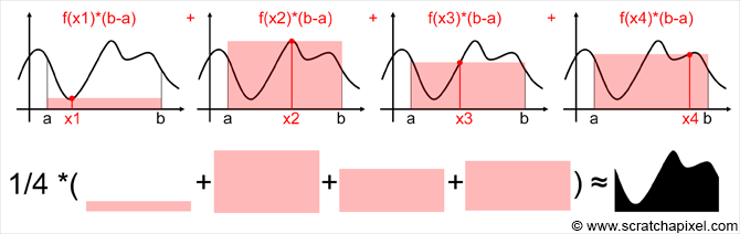
进一步来讲,其实从任意概率分布 $p_X(x)$ 中抽取样本 $f(X_{i})$,修正后的样本 $g(X)$ 都会趋近于目标积分值,这可以很容易的从前面的推导中得到:
可以将其记作:
因此虽然修正样本 $\cfrac{f\left(X\right)}{p(X)}$ 的形式有点奇怪,但随着样本越来越多,它将直接趋近积分值 $I$。考虑到我们使用蒙特卡洛方法主要就是用来估算积分,那么这个形式更直接了。
总之接下来可以放心的用 $\cfrac{f\left(X_{i}\right)}{p(X_{i})}$ 对积分做估计。
重要性采样
通过使用 $g(X)=\cfrac{f\left(X_{i}\right)}{p(X_{i})} $ ,我们可以从任意概率分布 $p_X(x)$ 中抽取样去估算积分值,那么不同的概率分布 $p_X(x)$ 会带来什么影响呢?
还是先从均匀采样的情况来看:
虽然这组估计值最终会趋近于积分值,但是估计值之间的差异可能很大
均匀采样时每个积分估计值 $g(x_{i}) $ 之间的差异将正比于函数值 $f(x_{i}) $ 的差异,当函数 $f(x)$ 本身差异很大时,虽然所有估计值都围绕着积分值分布,但不同样本的差异也会很大:有的估计值很大,有的估计值很小,这可能就需要用大量的样本才能让样本均值接近积分值。
例如用均匀采样对上一节材质特性中的光泽镜面反射做估计,大部分方向上对积分的估计值都是 $0$,这显然是不对的:
在均匀采样光泽镜面反射的方向时,大部分方向对积分的估计值都是 $0$
考虑另一种情况,假如概率分布 $p_{X}(x)$ 完全匹配目标函数 $f(x)$ 的话,那么每个概率值 $p_{X}(x_{i})$ 的大小就等于对应函数值 $f(x_{i})$ 占整个积分值的比重:
这将会有个不可思议的结果:只需要采样任意一个样本点 $X_{i}$,就可以得到精确的积分值:
或者说每个修正样本 $g(X_{i}) = \cfrac{f\left(X_{i}\right) }{ p(X_{i}) } $ 都是对积分值的完美估计。
只看左边的图,黄颜色的 $f(x)$ 是我们想求的积分,红颜色的 $p(x)$ 代表每个样本 $X_{i}$ 的概率密度函数,当 $p(x)$ 完全匹配 $f(x)$ 时,完美的估计就诞生了
当然这实际上是做不到的,因为 $ I$ 就是我们想要知道的值,在实际求解前它是未知的。但其实不需要完全匹配,只要两者能尽量匹配上,那么不说单样本求解积分,至少会比均匀采样好得多。因为这样每个修正样本 $g(X_{i}) = \cfrac{f\left(X_{i}\right) }{ p(X_{i}) } $ 都会非常的接近积分值 $I$ (只比积分值稍大一些或者稍小一些),那么同样的样本数量下,它们的均值也会更接近分值 $I$ 。
当使用的概率分布函数 $p_X(x)$ 能较好匹配目标函数 $f(x)$ 的 时,每个样本估计值都会更接近积分值
这样的采样方式被称为重要性采样 Importance Sampling。
最后再来回顾一下基于修正样本 $g(X) = \cfrac{ f\left(X\right) }{ p(X) } $ 直接估计函数积分值的做法,首先概率分布函数 $p_X(x)$ 的选取可以是任意的,根据之前的推导,最终样本均值都可以收敛到期望值:
而对于不同的概率分布函数 $p_X(x)$,在均匀采样的情况下起码能用,在概率分布 $p_X(x)$ 接近目标函数 $f(x)$ 时会非常好用,而且哪怕碰到了下图中甚至去反向匹配的概率密度函数,当样本数量数量足够多时,它仍然会趋近于真实值(比如说给比较大的函数值很小的采样概率,那么虽然很少会采样到这个函数值,但是一旦采样到了,就会产生非常大的估计值,抵消了极少样本的问题)。
均匀概率分布起码能用,能匹配上目标函数的概率分布将会非常好用,而即便碰到最右边的概率分布,$g(X) $ 仍然会趋近于积分值 $I$,只是需要更多的样本数量
通过修正过的样本 $g(X) = \cfrac{ f\left(X\right) }{ p(X) } $ 和重要性采样,我们可以根据材质特征更好的去放置样本点了。
Radiance(...) #2:采样 BRDF
先回顾一下之前对渲染方程做蒙特卡洛积分的做法:
(在这里 $\Omega = H^{2}(n)$,$L_{\mathrm{e}} = L_{\mathrm{emit}}$,$L_{\mathrm{i}} = L_{\mathrm{input}}$)
在之前的例子中,其实没有去考虑每个样本可能出现的概率,都是按均等概率抽取样本的:
现在有了更好的做法:
当令 $N=1$ 时:
现在唯一的问题是 $p(\omega_{\mathrm{i}})$ 要如何计算。
首先是不可能提前知道沿每个方向的入射光所反射能量
是多少的。
但是根据上一节材质表面反射分布的特性,可以想象假如现在只有一条光线击中了表面,那么
- 在镜面反射的情况下,它一定会从反射方向上离开;
- 对于光泽表面,它大概率会在反射方向的附近上离开;
- 对于漫反射表面,我们希望它从法线附近离开,因为在法线附近,入射光反射的亮度会比较高。
虽然不可能匹配到半球上所有入射光反射亮度的分布,但是可以去匹配 BRDF 的分布,只要比较接近就可以提高效率。
采样镜面反射分布
之前我们已经得到了镜面反射分布的 BRDF 为:
对镜面反射的采样非常简单,只在反射方向上采样,对应的概率分布函数为:
因此对镜面反射光的估计量为
这样做其实是为了把镜面反射这种特殊情况也统一到这个蒙特卡洛估计量里。
采样漫反射分布
由于漫反射分布的 BRDF 为
对应入射光的反射能量为
如果直接对这个 BRDF 进行采样,那就又回到了均匀采样上,在这种情况下我们可以对上式中的余弦项进行采样:
其中 $c$ 是一个归一化系数。根据
有
求解得到
于是
当光线在漫反射表面围绕法线方向出射时,所对应的一维概率分布的情况,我们希望大部分的样本集中在法线附近,这样可以更快的收敛到真实值
因此对漫反射光的单样本估计量为
......等等,这不就是 smallpt 的代码吗?
经历了又一大堆的铺垫后,我们在估计效率上往前进了一步,却发现 smalpt 早早在那候着了。
再来看看 smallpt 的原版代码:
   // line74~81
   if (obj.refl == DIFF){                  // Ideal DIFFUSE reflection
     double r1=2*M_PI*erand48(Xi), r2=erand48(Xi), r2s=sqrt(r2);
     Vec w=nl, u=((fabs(w.x)>.1?Vec(0,1):Vec(1))%w).norm(), v=w%u;
     Vec d = (u*cos(r1)*r2s + v*sin(r1)*r2s + w*sqrt(1-r2)).norm();
     return obj.e + f.mult(radiance(Ray(x,d),depth,Xi));

   } else if (obj.refl == SPEC)            // Ideal SPECULAR reflection
     return obj.e + f.mult(radiance(Ray(x,r.d-n*2*n.dot(r.d)),depth,Xi));
非常简洁的实现了重要性采样。
其中在漫反射的情况下,出射光线需要通过余弦加权进行采样(也就是注释里写的那样),至于说为什么那两行代码就可以做到余弦加权采样,具体推导请参考 PBRT 13.6.3。
不得不说 smallpt 的实现真巧妙,运行一下那只有 99 行的原版代码,你就会发现 编译不过 栈溢出了🤣。
Radiance(...) #3:终止条件
本以为可以结束对 Radiance() 函数的分析了,但它是个递归函数,还没有给终止条件🙄,好在下面的篇幅不那么长了。
回到渲染方程中,上文提到过它其实是一个递归方程:
在使用单样本采样估算积分时,每根光线经历一定的递归次数后,会得到一条光线路径
其中 $L_{\mathrm{i}} = L_{\mathrm{input}}$,$L_{\mathrm{o}} = L_{\mathrm{output}}$,$L_{\mathrm{e}} = L_{\mathrm{emit}}$。
在不考虑能量损耗的情况下,相机发射的光线可以在一个封闭空间中不停的穿梭,对应到这个方程中就是它会一直递归下去。
虽然我们可以通过蒙特卡洛方法去估算右边的积分了,但是要如何终止这个递归呢?
最简单的办法是达到一定的递归深度就终止,也就是只允许一条光线在空间中穿梭有限次。但这个深度如果太小就可能丢失掉一些重要路径(比如多次镜面反射),太大又非常浪费(多次漫反射)。至少一个固定的路径长度并不理想。况且相比于前面无偏差的单样本估计,这个方案并不优美,它违背了真实物理法则。
那么有没有一个办法,可以在有限次数的计算里去估算这个可能无穷深度的递归呢?(蒙特卡洛方法:谁又在叫我?)
再回到我们熟悉的一维积分中:
继续用蒙特卡洛方法来估算这个积分:
假如这里的函数 $ f(x) $ 非常复杂,每次计算都需要极高的代价,那么能不能在保持无偏的情况下减少用来估算的样本呢?
首先对于原积分,可以用一个比例 $P \ (0 < P <= 1) $ 去缩小定义域(同时放大对应的函数值),会得到一个新的积分:
两者的积分值是相同的
这样新积分 $ I_{P}$ 的积分值仍然等同于原积分 $ I$。
借助这种缩放的想法,可以在原来的定义域 $[0, 1] $ 中构造出一个新的蒙特卡洛估计量:
其中
也就是说只有当每个随机样本的样本值小于比例 $ P $ 时,才使用这个样本,否则丢弃掉它,此时 $\hat{I}_{RR} $ 的期望值为:
因为此时每个随机样本 $X_{i} $ 相当于是从区间 $[0, P]$ 中取均匀抽取出来的,所以 $\hat{I}_{RR} $ 的期望等同于 $\hat{I} $ 的期望,仍然是无偏的。
乍一看这好像没什么用,想减少样本的话在估算开始设定一下不就行了。但是考虑到上面计算期望的过程中,每个样本的期望是可以独立计算的,那么比例 $P$ 其实也是独立的,我们根据每个样本 $X_{i}$ 的特征,去设计单独的比例 $P_{X_{i}} \ (0 < P_{X_{i}} <= 1) $,那么 $\hat{I}_{RR} $ 的期望又变成了:
因此我们得到了一种可以在抽样过程中,动态评估是否计算一个样本的算法。上面这个算法被称为俄罗斯轮盘赌(Russian Roulette)。
那么这有什么用呢?
回到之前的问题中,对于光线在场景中发生多次镜面反射的情况,我们希望有比较长的光线路径;对于多次漫反射的情况,则希望尽快终止它;使用一个固定的路径长度并不合适,最好能根据不同路径的特点,自适应的去判断。
考虑到这么判断的原因是不同路径返回的亮度大小不同(同一个光源,通过镜面反射返回的亮度大,通过漫反射返回的亮度小),那么不妨根据 $f^{\prime}(X_{i}) $ 的做法,将 $ \hat{ L_{\mathrm{i}}\left(\mathrm{p}, \omega_{\mathrm{i}}\right) } $ 改造成 $ \hat{ L^{\prime}_{\mathrm{i}}\left(\mathrm{p}, \omega_{\mathrm{i}}\right) }$:
其中 $P$ 取 $f_{r}\left(\mathrm{p}, \omega_{\mathrm{o}}, \omega_{\mathrm{i}}\right)$ 的最大分量,以及
在这里,通过轮盘赌的路径会返回更多的亮度,以此抵消缩短的路径长度。
再来看 smallpt_comment.cpp 的代码:
    Color f = obj.color; // bsdf value
    double max_component = std::max({ f.x, f.y, f.z }); // max refl

    //russian roulette
    if (++depth > 5)
    {
        if (erand48(sampler) < max_component)
            f = f * (1 / max_component);
        else
            return obj.emission;
    }
其实 smallpt 已经加上了这个优化,并且还设定了要在路径至少达到一定深度后才开始轮盘赌。
那为什么还发生栈溢出了?
因为轮盘赌只是按一定概率去终止路径,那么就可能存在一直没有被终止的路径。
在理想的没有能量损耗的情况下,光线在两个镜面之间不停的来回穿梭
看来一圈折腾下来还是没完全解决问题,那么就做出必要的,工程实践上的取舍好了:路径过长时,强制终止。
    double distance; // distance to intersection
    int id = 0; // id of intersected object

    if (!Intersect(ray, distance, id))
        return Color(); // if miss, return black

    const Sphere& obj = Scene[id]; // the hit object

    if (depth > 10)
        return obj.emission; // if path is too long, only return sphere's emission
Radiance(...) #4:菲涅尔镜面散射
除此之外,smallpt 中还有第三种,会在光滑表面上同时发生反射和折射的材质类型,这背后涉及到了折射定律及全内反射(Total Internal Reflection,TIR),菲涅尔方程及其近似 Schlick's approximation。
这一块的内容也相当重要,有大量相关的资料讨论,同时本节到目前的篇幅实在太长,就不再展开介绍了。
这里提一个 Schlick's approximation 的实现细节:
其中余弦角 $\cos \theta$ 一般是根据入射光线及表面法线的夹角 $\theta_{\mathrm{i}}$ 得到的,
然而当光线从光密物质进入光疏物质时, 需要使用 $\theta_{t} $ 作为参数
Computer Graphics: Principles and Practice 3rd Chapter 26.5, Chapter 27.8.1
这样, 当快要接近全内反射的时候, $\theta_{t} $ 也就快要接近 90 度, 返回的 $R_F(\theta)$ 将会接近 1。
对应 smallpt_comment.cpp 的代码:
        // line 242~250
        // compute the fraction of incoming light that is reflected or transmitted
        // by Schlick Approximation of Fresnel Dielectric 1994 https://en.wikipedia.org/wiki/Schlick%27s_approximation
        double a = etaT - etaI;
        double b = etaT + etaI;
        double R0 = a * a / (b * b);
        double c = 1 - (into ? -cosThetaI : refractDirection.Dot(normal));

        double Re = R0 + (1 - R0) * c * c * c * c * c;
        double Tr = 1 - Re;
本节总结
🙄这里为了能把这个 radiance(...) 函数讲清楚,费了相当多的笔墨周折(哪怕这样都还省略了一些内容),不过接下来把 samllpt 改写成 PBRT 的部分就很直观了。
另外 radiance(...) 是个尾递归函数,有兴趣的同学可以尝试把它改成迭代的看看。
改写 smallpt
这一步会把 smallpt 改写成 pbrt,在改写之前先来介绍下 pbrt。
pbrt 的主要功能是根据输入的描述文件创建出场景,并根据相机的参数渲染出对应图像,它的整个工作过程如下:

SamplerIntegraotr:通过(蒙特卡洛方法)采样,来求解渲染方程(一个积分方程的)的积分器,也可以把它当做通常的渲染器 Renderer 看待。SamplerIntegraotr::Render(): SamplerIntegraotr 的基类是抽象类 Integrator,它只有Integraotr::Render()这一个接口,pbrt 在创建完场景和积分器后,就会调用积分器开始渲染场景。每种积分器实现会用自己的方式去渲染场景。- 对于 SamplerIntegraotr::Render() 来说,它也会遍历图像平面 Film,通过采样器 Sampler 在图像的每个像素上生成相机要用的采样点 CameraSample ,然后传递给相机 Camera 生成光线 Ray ,寻找光线到场景 Scene 中的最近交点 Intersection ,在交点上计算半球积分,返回沿光线方向辐射出的亮度……与 smallpt 的主函数 main() 如出一辙。
SamplerIntegraotr::Li(): SamplerIntegraotr 的核心方法是Li(ray, scene, sampler, depth),对应 smallpt 中的Radiance(ray, sampler, dpeth)(smallpt 的场景是全局的,不用传进来)。在 Li(ray, scene, sampler, depth) 中会同时采样 BRDF 和光源,关于要如何采样光源,会放到额外拓展的部分介绍。

这就是 pbrt 的整体架构,也是 pbrt 的核心功能:求解渲染方程。(smallpt:我也是)
是不是对上了。
对于上面描述的这些概念,pbrt 都有对应的抽象类(接口类)来实现:

并且通过这组抽象类之间的交互(上面的箭头)来完成功能。每个抽象类都会有多种实现,比如对于材质 Material,就可以有哑光材质 MatteMaterial(通过完全漫反射 BRDF LambertenReflection 实现);镜面材质 MirrorMaterial(通过完全镜面反射 BRDF SpecularReflection 实现)。这些实现类基本放在 core/ 之外的其它文件夹下。
除此之外 pbrt 还实现了大量别的功能:并行/内存分配/统计/调试/场景解析等一系列功能,于是它的代码行数就来到了几万行(没统计过,大概是这个量级)。
99 行 vs 几万行,这两个数量级要怎么跨过呢?
给 smallpt 加功能是不可能的,假如只保留 pbrt 的核心功能,去掉那些实现类和其它功能呢?
- 不需要那么多种几何形状,球体 Sphere 就够了:去掉
shape/目录 - 不需要那么多种相机,透视相机 PerspectiveCamera 就够了:去掉
camera/目录 - 不需要那么多种采样器,最基本的随机采样器 RandomSampler 就够了:去掉
sampler/目录 - ……
至于场景中的空间加速结构 Aggregate,图像平面的滤波器 Filter,提供材质细节的纹理 Texture,实现体积渲染的介质 Medium 等,连抽象类都可以去掉。
到这里就只剩下了 core/ 这个目录,把它的代码整合一下,再去掉并行等一系列没了也能跑的功能,给每个抽象类(Shape,Sampler,Camera,BSDF/BxDF,Light,Integrator……)加上最简单的实现,我们就得到了一千行左右的 smallpt_rewrite.cpp。(也可以管它叫 smallpbrt.cpp )
如果在这个基础上再做精简的话:
- 类结构也不要了:smallpt_comment.cpp (因此在 samllpt 里看不到 Sampler,Camera 这些类,但功能还在 )
- 代码级别的结构和变量命名也不要了:smallpt_format.cpp (这个
Radiance(...)的实现都是 tirck 吧) - 再压缩一下行数:smallpt.cpp
- 把带有菲涅尔反射的材质也去掉:nanopt.cpp
- 收手吧
在前几节,我们已经从 smallpt.cpp 反向实现了 smallpt_format.cpp 和 smallpt_comment.cpp ,接下来将把 300 行的 smallpt_comment.cpp 结构化为 1300 行的 smallpt_rewrite.cpp / smallpbrt.cpp ,这就有了本文的标题。
smallpt_rewrite.cpp 的提交记录比较干净,感兴趣的同学可以直接看每次提交都结构化了什么功能。
下面开始改写吧
因为 Shape,Material,Light 的功能目前都交织在一起,并不好修改,所以会把它们留到最后。
最开始先来改写主函数 main() 。
胶片/图像平面 Film
最开始结构化是 Film 这个类,因为 smallpt 目前使用了 ppm 格式来保存图像,很多图像软件都不支持这种格式,所以先换成用 bmp 格式来保存,这样在每次渲染完以后就可以用 WIndows 自带的画图软件来自动打开图像。
Film 封装了累加颜色,保存图像的功能,本身比较简单(关于 bmp 图像的格式这里就不做介绍了)。其中保存图像的接口是参考 stb_image_write.h 来设计的,感兴趣的同学很容易换成其他格式来保存。
/*
  warpper of `Color pixels[]`
  features:
    * get/set color
    * save image
*/
class Film
{
public:
    Film(const Vector2& resolution, /*std::unique_ptr<Filter> filter,*/ const std::string& filename) :
        fullResolution{ resolution },
        filename{ filename },
        pixels{ std::make_unique<Color[]>(Width() * Height()) }
    {
    }

public:
    int  Width() const { return (int)fullResolution.x; }
    int Height() const { return (int)fullResolution.y; }
    Vector2 Resolution() const { return fullResolution; }

    Color& operator()(int x, int y)
    {
        return *(pixels.get() + Width() * y + x);
    }

    void add_color(int x, int y, const Color& delta)
    {
        Color& color_ = operator()(x, y);
        color_ = color_ + delta;
    }

public:
    virtual bool store_image() const
    {
        return store_bmp_impl(filename, Width(), Height(), 3, (Float*)pixels.get());
    }

    // ...

private:
    const Vector2 fullResolution;
    //std::unique_ptr<Filter> filter;
    const std::string filename;

    std::unique_ptr<Color[]> pixels;
};
pbrt 里 Filter,Film 的实现
Filter 和 Film 在 PBRT 的第 7.8, 7.9 节先后进行了描述。
在 pbrt 的 Film 中还保存了每个像素的权重信息,用来在渲染结束后做图像平面做滤波,不过这里的实现很简单,因此也没有加入滤波器 Filter。
因为 pbrt 支持多线程渲染,为了避免多个线程同时往 Film 里写入数据,就增加了一个 FilmTile 类,表示 Film 中的一块区域。每个线程在渲染时使用单独的 FilmTile(以及单独的 Sampler 和负责分配内存的 MemoryArena ),在渲染完这块区域后将 FilmTile 里的数据合并回 Film 中,总体来说比较琐碎。以上细节笔者有记录过,感兴趣的同学可以看 这里。
至于如何将每个像素中的光谱值保存为颜色值,则涉及到 PBRT 第 5 章的内容,这里先不展开了。
采样器 sampler
随机数生成器 RNG
// random number generator
// https://github.com/SmallVCM/SmallVCM/blob/master/src/rng.hxx
class RNG
{
public:
    RNG(int seed = 1234) : rngEngine(seed)
    {
    }

    // [0, 1)
    Float UniformFloat()
    {
        return float01Dist(rngEngine);
    }

    // [0, 1), [0, 1)
    Float2 UniformFloat2()
    {
        return Float2(UniformFloat(), UniformFloat());
    }

private:
    std::mt19937_64 rngEngine;
    std::uniform_real_distribution<Float> float01Dist{ (Float)0, (Float)1 };
};
其中 MT1994 是一个伪随机数生成器(基于梅森旋转算法),这里使用一个固定的种子来出初始化,是为了方便后面的调试。在 smallpt_rewrite.cpp 里只使用这个 RNG 生成 0~1 之间均匀分布的浮点型随机数。
采样器接口
class Sampler
{
public:
    virtual ~Sampler() {}
    Sampler(int samplesPerPixel) :
        samplesPerPixel{ samplesPerPixel }
    {
    }

    virtual int SamplesPerPixel()
    {
        return samplesPerPixel;
    }

    virtual std::unique_ptr<Sampler> Clone() = 0;

public:
    virtual void StartPixel()
    {
        currentSampleIndex = 0;
    }

    virtual bool StartNextSample()
    {
        currentSampleIndex += 1;
        return currentSampleIndex < samplesPerPixel;
    }

public:
    virtual Float Get1D() = 0;
    virtual Vector2 Get2D() = 0;
    virtual CameraSample GetCameraSample(Point2 pFilm) = 0;

protected:
    RNG rng{};

    int samplesPerPixel{};
    int currentSampleIndex{};
};
这里只包含 pbrt 中采样器的部分接口。
在使用这个采样器替换了 smallpt 里采样相关的逻辑后,主函数里的 5 个 for 循环降到了 2 个,从每个像素中采样多少个相机样本的逻辑也交给了 sampler 来控制。原先生成相机样本的逻辑被放到了 TrapezoidalSampler 里,考虑到这个实现看起来有点复杂和奇怪,笔者还加入了更简单的随机采样器 RandomSampler:
class RandomSampler : public Sampler
{
public:
    using Sampler::Sampler;

    std::unique_ptr<Sampler> Clone() override
    {
        return std::make_unique<RandomSampler>(samplesPerPixel);
    }

public:
    Float Get1D() override
    {
        return rng.UniformFloat();
    }

    Vector2 Get2D() override
    {
        return rng.UniformFloat2();
    }

    CameraSample GetCameraSample(Point2 pFilm) override
    {
        return { pFilm + rng.UniformFloat2() };
    }
};
*pbrt 里的的 RNG 和 Sampler
RNG 在附录部分进行了简要介绍。
Sampler 在第 7 章进行了介绍,它对于整个系统来说至关重要,好的采样器可以大幅减少蒙特卡洛光线追踪里需要的样本数,也就缩短了渲染时间,坏的采样器则可能导致错误的渲染结果。
除了伪随机数外,pbrt 里还是用了拟随机数( Quasi random numbers),这是一种完全确定的,具有规律的“随机数”,对应的蒙特卡洛算法称为 拟蒙特卡洛( Quasi Monte Carlo)。在蒙特卡洛光线追踪中,拟随机数 QRNG 比伪随机数 PRNG 更好用,这是个有点意外的结果。
对于笔者这个没学过信号处理,采样理论的人来说,这一章着实难懂。在不了解整体框架下,Sampler 的其它接口也很难懂(建议以后再看的注释)。有个简单的办法就是先忽略掉它们,暂且用 RandomSampler 理解整个渲染的流程。
相机 Camera
/*
  pbrt camera space:
    left hand
  y (0, 1, 0)         z(0, 0, 1)
        |            /
        |          /
        |        /
        |      /
        |    /
        |  /
        |/_ _ _ _ _ _ x(1, 0, 0)
        o
  features:
    generate ray
*/
class Camera
{
public:
    virtual ~Camera() {}
    Camera() {}

public:
    virtual Ray GenerateRay(const CameraSample& sample) const = 0;
};
相机是个很简洁的接口类,它只负责根据图像平面的样本点,生成光线。
因为 pbrt 用的是左手系,而 smallpt 使用了右手系,所以这次提交还把场景翻转了一下🙃。
这里将 smallpt 里的透视相机替换成了这个比较常规的实现:
// https://github.com/infancy/pbrt-v3/blob/master/src/cameras/perspective.cpp
class PerspectiveCamera : public Camera
{
public:
    PerspectiveCamera(const Vector3& position, const UnitVector3& direction, const Vector3& up,
        Degree fov, Vector2 resolution) :
        position{ position },
        front{ direction },
        up{ up },
        resolution{ resolution }
    {
        // `front` is a unit vector, it's length is 1
        Float tan_fov = std::tan(radians(fov) / 2);

        right = this->up.Cross(front).Normalize() * tan_fov * Aspect();
        this->up = front.Cross(right).Normalize() * tan_fov;
    }

public:
    virtual Ray GenerateRay(const CameraSample& sample) const
    {
        Vector3 direction =
            front +
            right * (sample.pFilm.x / resolution.x - 0.5) +
            up * (0.5 - sample.pFilm.y / resolution.y);

        return Ray{ position + direction * 140, direction.Normalize() };
    }

private:
    Float Aspect() { return resolution.x / resolution.y; }

private:
    Vector3 position;
    UnitVector3 front;
    UnitVector3 right;
    UnitVector3 up;

    Vector2 resolution;
};
pbrt 里的相机
相机模型在第 6 章进行了介绍。这一章除了基本的相机模型,常用的透视投影相机和正交投影相机外,还介绍了跟踪相机位置上所有方向的环境相机 EnvironmentCamera(可以用来生成环境贴图),和模拟真实世界中具有复杂透镜结构的真实相机 RealisticCameras。
至于 pbrt 中的 Camera,它使用矩阵对光线做变换,同时拥有更多的接口,其中 GenerateRayDifferential 生成的光线可以用来做纹理过滤,不过我们没用到纹理,暂时也可以忽略掉它和 RayDifferential。
至于其它三个接口,因为 pbrt 除了对 BRDF 和光源进行采样外,还会对相机进行采样,那时才会用到它们,不过这是进阶算法才会做的事情,在当前阶段可以忽略掉它们。
class Camera {
  public:
    // Camera Interface
    Camera(const AnimatedTransform &CameraToWorld, Float shutterOpen,
           Float shutterClose, Film *film, const Medium *medium);
    virtual ~Camera();

    // 返回世界空间中的 ray, ray 是经过归一化的, 整个系统依赖于这个行为
    // 最后返回的浮点值代表在 film 上的贡献值, 用来模拟真实相机的渐晕效果
    virtual Float GenerateRay(const CameraSample &sample, Ray *ray) const = 0;

    // 在 GenerateRay 生成的主光线的基础上, 往胶片平面的x,y方向上各偏移一像素生成辅助光线
    // 生成的 RayDifferential 结构主要用于纹理反走样
    virtual Float GenerateRayDifferential(const CameraSample &sample,
                                          RayDifferential *rd) const;

    // used in Section16, bidirectional light transport algorithms
    virtual Spectrum We(const Ray &ray, Point2f *pRaster2 = nullptr) const;
    virtual void Pdf_We(const Ray &ray, Float *pdfPos, Float *pdfDir) const;
    virtual Spectrum Sample_Wi(const Interaction &ref, const Point2f &u,
                               Vector3f *wi, Float *pdf, Point2f *pRaster,
                               VisibilityTester *vis) const;

    // Camera Public Data
    // P356
    AnimatedTransform CameraToWorld; // 可以把相机变换到世界空间中
    const Float shutterOpen, shutterClose; // 快门时间, 用于模拟运动模糊
    Film *film;
    const Medium *medium;
};
改到这里,主函数暂且就这样,我们已经有 Film,Sampler 和 Camera,可以生成光线,去改造 Radiance(...) 函数了。
表面着色 Shading
在改写 Radiance 函数之前,先回顾一下只考虑直接光照时,表面着色需要做些什么:
- 找到最近的交点,计算交点上的信息
- 几何属性:世界空间中的位置 $\mathrm{p}$,法线方向 $\mathrm{n}$,光线入射的方向 $\omega_\mathrm{o}$。
- 材质属性:从当前交点对应的物体中获取材质信息,并计算出交点上的 BRDF。
- 光照属性:物体是否存在自发光。
- 遍历交点半球方向上的所有光源,累计所有可见光在 $\omega_\mathrm{o}$ 方向上反射的亮度,并加上交点朝 $\omega_\mathrm{o}$ 方向上的自发光(假如有的话),将所有出射光沿 $\omega_\mathrm{o}$ 方向返回。
不过在 smallpt 里没有实现采样光源的功能,第二步就换成了在交点的整个半球方向上计算所有光照。
总之每次做着色时,焦点都在交点 Isect 上,它包含了着色所需要的所有信息,我们不需要再去关注交点对应的几何形状,材质等信息了。
在 smallpt.Radiance(...) 中,光线传输和表面着色这两件事是混在一起的,现在我们从交点 Isect 开始把它俩解耦开,方便后面两边独立的修改。
表面交点 Isect
根据上面的描述,这里实现了交点类 Isect,它会在光线求交的阶段生成,记录了在后续着色中需要的各种信息。因为不做纹理采样,所以没有求解纹理坐标的步骤。
有了交点类后,查询球体交点的接口变成了 bool Intersect(Ray& ray, Isect* isect),相比之前更简洁。
class BSDF;
class Primitive;

/*
class BSDF;
class Primitive;

/*
  surface intersection, called `SurfaceInteraction` on pbrt

  prev   n   next
  ----   ^   ----
    ^    |    ^
     \   | θ /
   wo \  |  / wi is unknown, sampling for bsdf (or light)
       \ | /
        \|/
      -------
       isect
*/
class Isect
{
public:
    Isect() = default;
    Isect(const Point3& position, const Normal3& normal, UnitVector3 wo) :
        position{ position },
        normal{ normal },
        wo{ wo }
    {
    }

public:
    Point3 position{}; // world position of intersection
    Normal3 normal{};
    UnitVector3 wo{};

    const BSDF* bsdf() const { return bsdfPtr.get(); }
    Color Le() const { return emission; } // prev <- isect, against ray's direction

private:
    std::unique_ptr<BSDF> bsdfPtr{};
    Color emission{};

    friend Primitive;
};
pbrt 中的表面交点 SurfaceInteraction
在第 2.10 节进行了介绍。因为 pbrt 还要做纹理采样,并且支持凹凸贴图(Bump Mapping),所以比这里的实现更复杂。
反射分布 BRDF
接下来是 Radinace(...) 中材质、BRDF 相关的功能:
    if (isect.materialType == MaterialType::Diffuse) // Ideal Diffuse reflection
    {
        // ...
    }
    else if (isect.materialType == MaterialType::Specular) // Ideal Specular reflection
    {
        // ...
    }
    else // Ideal Dielectric Refraction
    {
        // ...
    }
但它同时又包含了光线传输的逻辑,下面先用单独的 BSDF 类将着色功能分离出来。
首先定义的是用于重要性采样的样本结构,包含对 BSDF 进行采样得到的反射率/散射率 $f$,出射方向 $\omega_{\mathrm{i}}$ 和对应概率 $pdf$ :
struct BSDFSample
{
    Color f; // scattering rate
    Vector3 wi; // world wi
    Float pdf{};
};
接着是通过着色点法线计算得到的切线空间,或者说着色空间 Frame:
// https://github.com/SmallVCM/SmallVCM/blob/master/src/frame.hxx
class Frame
{
public:
    Frame(const Normal3& n) :
        n_{ n.Normalize() }
    {
        SetFromZ();
    }

public:
    Vector3 ToLocal(const Vector3& worldVec3) const
    {
        return Vector3(
            Dot(s_, worldVec3),
            Dot(t_, worldVec3),
            Dot(n_, worldVec3));
    }

    Vector3 ToWorld(const Vector3& localVec3) const
    {
        return
            s_ * localVec3.x +
            t_ * localVec3.y +
            n_ * localVec3.z;
    }

private:
    // world frame basic vector
    Vector3 s_{ 1, 0, 0 }; // x
    Vector3 t_{ 0, 1, 0 }; // y
    Normal3 n_{ 0, 0, 1 }; // z
};
其中省略了部分实现。
在 smallpt 中,所有计算都是在世界空间中完成的。而在 pbrt 中,因为有变换矩阵的存在,所有操作都可以先在本地空间(Local World)中先完成,再变换到世界空间或其它空间中。在本地空间中,很多涉及到坐标和方向的计算都可以被简化。
因为 BSDF 里只会涉及方向向量的计算,不需要完整的变换矩阵,只用三个相互正交的坐标轴就可以实现向量在世界空间和本地空间之间的变换。
最后是 BSDF 抽象类,它是在光线求交时,通过物体表面的材质属性生成的(目前还没有实现材质,依靠临时代码实现),在 smallpt_rewrite.cpp 里的主要作用就是在交点的半球方向上进行重要性采样,生成用于着色和光线传输的 BSDFSample 结构:
/*
  https://www.pbr-book.org/3ed-2018/Reflection_Models#x0-GeometricSetting


  shading frame:

       z, n(0, 0, 1)
       |
       |
       |
       |
       |_ _ _ _ _ _ x, s(1, 0, 0)
      / p
     /
    /
   y, t(0, 1, 0)
*/

class BSDF
{
public:
    virtual ~BSDF() = default;
    BSDF(Frame shadingFrame) :
        shadingFrame{ shadingFrame }
    {
    }

public:
    // or called `eval`, `evaluate`
    Color f(const Vector3& world_wo, const Vector3& world_wi) const
    {
        return f_(ToLocal(world_wo), ToLocal(world_wi));
    }

    Float Pdf(const Vector3& world_wo, const Vector3& world_wi) const
    {
        return Pdf_(ToLocal(world_wo), ToLocal(world_wi));
    }

    // or called `sample`, `sample_direction`
    BSDFSample Sample_f(const Vector3& world_wo, const Float2& random) const
    {
        auto sample = Sample_f_(ToLocal(world_wo), random);
        sample.wi = ToWorld(sample.wi);

        return sample;
    }

protected:
    virtual Color f_(const Vector3& wo, const Vector3& wi) const = 0;
    virtual Float Pdf_(const Vector3& wo, const Vector3& wi) const = 0;

    virtual BSDFSample Sample_f_(const Vector3& wo, const Float2& random) const = 0;

private:
    Vector3 ToLocal(const Vector3& worldVec3) const
    {
        return shadingFrame.ToLocal(worldVec3);
    }

    Vector3 ToWorld(const Vector3& localVec3) const
    {
        return shadingFrame.ToWorld(localVec3);
    }

private:
    Frame shadingFrame;

    // extension point:
    // std::array<bxdf_uptr, 2> BxDFList;
};
这个抽象类主要负责对方向做变换,之后具体的计算可以在不同实现的着色空间里完成。
漫反射分布 LambertionReflection
它是完全按照之前在 Radiance(...) 中分析的内容来实现的:
class LambertionReflection : public BSDF
{
public:
    LambertionReflection(const Frame& shadingFrame, const Color& R) :
        BSDF(shadingFrame), R{ R }
    {
    }

    Color f_(const Vector3& wo, const Vector3& wi) const override { return R * InvPi; }

    Float Pdf_(const Vector3& wo, const Vector3& wi) const override
    {
        return SameHemisphere(wo, wi) ? CosineHemispherePdf(AbsCosTheta(wi)) : 0;
    }

    BSDFSample Sample_f_(const Vector3& wo, const Float2& random) const override
    {
        BSDFSample sample;

        // Cosine-sample the hemisphere, flipping the direction if necessary
        sample.wi = CosineSampleHemisphere(random);
        if (wo.z < 0)
            sample.wi.z *= -1;

        sample.pdf = Pdf_(wo, sample.wi);
        sample.f = f_(wo, sample.wi);

        return sample;
    }

private:
    Color R; // surface reflectance
};在应用它之后,Radiance(...) 对应的代码将由
    if (isect.materialType == MaterialType::Diffuse) // Ideal Diffuse reflection
    {
        Float random1 = 2 * Pi * sampler.Get1D();
        Float random2 = sampler.Get1D();
        Float random2Sqrt = sqrt(random2);

        // shading coordinate on intersection
        Vector3 w = shading_normal;
        Vector3 u = ((fabs(w.x) > .1 ? Vector3(0, 1, 0) : Vector3(1, 0, 0)).Cross(w)).Normalize();
        Vector3 v = w.Cross(u);

        // Cosine importance sampling of the hemisphere for diffuse reflection
        Vector3 direction = (u * cos(random1) * random2Sqrt + v * sin(random1) * random2Sqrt + w * sqrt(1 - random2)).Normalize();

        f = f / Pi; // for lambert brdf, f = R / Pi;
        Float abs_cos_theta = std::abs(shading_normal.Dot(direction));
        Float pdf = abs_cos_theta / Pi; // cosine-weighted sampling
        return isect.Le() + (f * Radiance(Ray(position, direction), depth, sampler) * abs_cos_theta) / pdf;
    }
变成
    if (isect.materialType == MaterialType::Diffuse) // Ideal Diffuse reflection
    {
        auto bs = isect.bsdf()->Sample_f(isect.wo, sampler.Get2D());
        if (bs.f.IsBlack() || bs.pdf == 0.f) // pdf == 0 => NaN
            return isect.Le();

        Ray wi(isect.position, bs.wi);
        return isect.Le() + (bs.f * Radiance(wi, depth, sampler) * AbsDot(bs.wi, isect.normal) / bs.pdf);
    }
采样的细节都被转移到 LambertionReflection 里了。
继续对剩下采样 BSDF 的功能做这个操作。
镜面反射 SpecularReflection
    else if (isect.materialType == MaterialType::Specular) // Ideal Specular reflection
    {
        Vector3 direction = ray.direction - normal * 2 * normal.Dot(ray.direction);
        return isect.Le() + f * Radiance(Ray(position, direction), depth, sampler);
    }
else if (isect.materialType == MaterialType::Specular) // Ideal Specular reflection
{
auto bs = isect.bsdf()->Sample_f(isect.wo, sampler.Get2D());
Ray wi(isect.position, bs.wi);
return isect.Le() + (bs.f * Radiance(wi, depth, sampler) * AbsDot(bs.wi, isect.normal) / bs.pdf);
}菲涅尔镜面散射 FresnelSpecular
else // Ideal Dielectric Refraction
{
// ...
} else // Ideal Dielectric Refraction
{
auto bs = isect.bsdf()->Sample_f(isect.wo, sampler.Get2D());
Ray wi(isect.position, bs.wi);
return isect.Le() + (bs.f * Radiance(wi, depth, sampler) * AbsDot(bs.wi, isect.normal) / bs.pdf);
}现在采样 BSDF 的功能都被转移到 BSDF 里了。于是乎,我们得到了这样一串代码:
if (isect.materialType == MaterialType::Diffuse) // Ideal Diffuse reflection
{
auto bs = isect.bsdf()->Sample_f(isect.wo, sampler.Get2D());
if (bs.f.IsBlack() || bs.pdf == 0.f) // pdf == 0 => NaN
return isect.Le();
Ray wi(isect.position, bs.wi);
return isect.Le() + (bs.f * Radiance(wi, depth, sampler) * AbsDot(bs.wi, isect.normal) / bs.pdf);
}
    else if (isect.materialType == MaterialType::Specular) // Ideal Specular reflection
    {
        auto bs = isect.bsdf()->Sample_f(isect.wo, sampler.Get2D());

        Ray wi(isect.position, bs.wi);
        return isect.Le() + (bs.f * Radiance(wi, depth, sampler) * AbsDot(bs.wi, isect.normal) / bs.pdf);
    }
    else // Ideal Dielectric Refraction
    {
        auto bs = isect.bsdf()->Sample_f(isect.wo, sampler.Get2D());

        Ray wi(isect.position, bs.wi);
        return isect.Le() + (bs.f * Radiance(wi, depth, sampler) * AbsDot(bs.wi, isect.normal) / bs.pdf);
}因为所有 BSDF 的实现都使用了相同的接口,所以对它们做采样的方式也一样,不需要再去做区分了。于是我们可以对 Radiance(...) 做一次简化:
Color Radiance(Ray ray, int depth, Sampler& sampler)
{
    Isect isect;
    if (!Intersect(ray, &isect))
        return Color(); // if miss, return black

    if (depth > 10)
        return isect.Le();

    auto bs = isect.bsdf()->Sample_f(isect.wo, sampler.Get2D());
    if (bs.f.IsBlack() || bs.pdf == 0.f) // pdf == 0 => NaN
        return isect.Le();

    //russian roulette
    if (++depth > 5)
    {
        Float bsdf_max_comp = bs.f.MaxComponentValue();
        if (sampler.Get1D() < bsdf_max_comp) // continue
            bs.f = bs.f * (1 / bsdf_max_comp);
        else
            return isect.Le();
    }

    Ray wi(isect.position, bs.wi);
    return isect.Le() + (bs.f * Radiance(wi, depth, sampler) * AbsDot(bs.wi, isect.normal) / bs.pdf);
}
和原先比起来,现在它变得相当简洁了。
pbrt 中的 BSDF/BxDF
BSDF 在第 8 章进行了介绍。
pbrt 中实现了更多种类的 BSDF,并且允许交点上携带多种 BSDF,这是通过组合来实现的:
class BxDF;

class LambertionReflection: public BxDF;
class SpecularReflection: public BxDF;
class FresnelSpecular: public BxDF;
// ...

class BSDF
{
    // ...

    BxDF* bxdfs[MaxBxDFs];
};
为了保持单光线采样,pbrt 在采样 BSDF 时会先用蒙特卡洛方法从 bxdfs 中挑选一个出来作为样本,在 samllpt_rewrite.cpp 的菲涅尔镜面材质中也做了类似的操作。
场景 Scene
在渲染器中,场景主要提供了查询光线最近交点,光线到光源之间是否存在遮挡等功能,因为这里不采样光源,所以只提供光线求交的功能:
class Scene
{
public:
    Scene() = default;
    Scene(
        std::vector<std::shared_ptr<Shape>> shapeList, std::vector<std::shared_ptr<Material>> materialList, std::vector<std::shared_ptr<Light>> lightList, std::vector<Primitive> primitiveList) :
        shapeList{ shapeList },
        materialList{ materialList },
        lightList{ lightList },
        primitiveList{ primitiveList }
    {
    }

public:
    bool Intersect(Ray& ray, Isect* isect) const
    {
        bool bHit = false;

        for (const auto& primitive : primitiveList)
        {
            if (primitive.Intersect(ray, isect))
            {
                bHit = true;
            }
        }

        return bHit;
    }

public:
    static Scene CreateSmallptScene()
    {
        // ...
    }

private:
    std::vector<std::shared_ptr<Shape>> shapeList;
    std::vector<std::shared_ptr<Material>> materialList;
    std::vector<std::shared_ptr<Light>> lightList;

    std::vector<Primitive> primitiveList;
};
当前积分器只需要往场景里投射光线查询交点就好了,至于场景里的细节一概不需要了解。
因为这个场景非常简单,所以在求交的时候没有使用空间加速结构。
这里的 Primitive 将在下一节介绍。
pbrt 里的 Scene
在 附录B 中对场景描述文件,对每个对象的创建参数等一系列问题进行了讲解。
图元 Primitive
在最后一次提交中同时加入了 Shape, Material, Light, Primitive 四个抽象类,从表面着色那一节,我们知道了交点 Isect 需要诸多信息来进行着色,在 pbrt 里这些信息将全部由图元 Primitive(笔者更喜欢称呼它为表面 Surface) 给出:
struct Primitive
{
    const Shape* shape;
    const Material* material;
    const AreaLight* areaLight;

    bool Intersect(Ray& ray, Isect* isect) const
    {
        bool hit = shape->Intersect(ray, isect);
        if (hit)
        {
            isect->bsdfPtr = material->Scattering(*isect);
            isect->emission = areaLight ? areaLight->Le(*isect, isect->wo) : Color();
        }

        return hit;
    }
};
其中交点上的几何信息由具体的几何形状 shape 给出。
pbrt 中的 Primitive
在 4.1 节进行了介绍。
光源 Light
smallpt_rewrite.cpp 中只实现了区域光源 AreaLight,并且只提供了朝光线入射方向 $\omega_{\mathrm{o}}$ 返回自发光 $Le$ 的功能:
class Light
{
};

class AreaLight : public Light
{
public:
    AreaLight(Color radiance, const Shape* shape) :
        radiance{ radiance },
        shape{ shape }
    {
    }

    Color Le(const Isect& lightIsect, const Vector3& wo) const
    {
        return (Dot(lightIsect.normal, wo) > 0) ? radiance : Color();
    }

private:
    Color radiance;
    const Shape* shape;
};
pbrt 中的光源
在采样光源时时,pbrt 会和采样 BSDF 一样,先从一组光源里采样出光源的样本,再对这个光源进行采样。
*进一步拓展
当前的 smallpt_rewrite.cpp 已经初具规模了,但它和 pbrt 相比还有个很重要功能没有实现:采样光源。但是要把这部分功能加上的话,整个文件的体积和复杂性又会进一步增加。
为了保持 smallpt_rewrite.cpp 当前的简洁性,笔者把相关功能加在了另一个文件里:ky.cpp,从提交历史来看,它其实是最初的实验性作品,包含了最多的功能特性,并使用了另外一种代码风格,但目前仍未稳定(还有些临时代码和 bug),同时这里的内容相对难理解一点,因此下文只做简要介绍。
对光源采样
- 实现代码:
integrater_t::estimate_direct_lighting_position(...)
因为 samllpt 中没有包含对光源采样的实现,所以在讲解 Radiance(...) 时没有展开介绍这种做法,但是采样光源具有重要的意义,同时能极大的提升渲染速度。
回到 Radiance(...) 中介绍面积光源的那一段,我们有:
并且还把它拓展到了整个半球方向上进行采样,最终得到了全局光照效果。
现在往后退一步,先尝试去估算这个面积光源上的直接光照:
下文中将这个估计量记作 $ \hat{L_{\mathrm{o}}\left(\mathrm{p}, \omega_{\mathrm{o}}\right)}$。

首先这个估计有点奇怪,我们明明知道光源在哪,长什么样子,为什么不能让光线往光源的位置出射,反而要在半球方向上根据 BRDF 来选择方向呢?
进一步的,对于小型的面积光源,这样做的效率非常低。对于点光源,方向光源这样具有奇异分布的光源(类似于镜面反射 BRDF),则根本无法采样到它们,因此有必要直接去采样光源,下面仍以面积光源为例进行介绍。
首先方向 $\omega_{\mathrm{i}}$ 是很容易确定的,只需要在光源上随机采样一点 $\mathrm{P^{\prime} }$,那么从交点 $\mathrm{P} $ 到 $\mathrm{P^{\prime}}$ 的连线就是采样方向 $\omega_{\mathrm{i}}$。

其次要保证从交点 $\mathrm{P} $ 到光源采样点 $\mathrm{P^{\prime}}$ 之间无遮挡(这是在采样方向时不需要考虑的问题),这其实可以转化为 “对于光线 $\text{Ray} (\mathrm{P} , \ \mathrm{P^{\prime}}- \mathrm{P} ) $, 在整个场景中有没有比 $\mathrm{P^{\prime}}$ 更近的交点,有的话就说明存在遮挡”,那么遮挡问题就变成了已经实现的查询场景交点的问题。
可以把这个遮挡查询的操作记作
称其为可见函数(visibility function)或可见项(visibility term),它是一个只返回 0 或 1 的函数,0 表示两点之间存在遮挡,1 表示两点之间完全可见。
最后仍然是如何处理概率密度函数 $p( \omega_{\mathrm{i}} ) $,因为这一次是对光源进行采样,需要一种基于光源的 $p( \omega_{\mathrm{i}} ) $,在解决这个问题之前,先来说说投影面积和立体角。
投影面积和立体角
首先如下图所示,可以根据夹角的余弦值来计算投影面积:

因为光源不一定是正对着交点(法线)的,所以在计算光源对交点所形成的立体角时,也应该用投影面积来计算:
对应二维的情况, 这大概叫投影平面角?
立体角建立了半球方向上的面积和立体角之间的转换关系,它可以用来计算面积光源在交点半球方向上的投影立体角大小,使我们可以先采样光源中某一点,再将它转化回立体角。这样直接采样光源可以极大的提升渲染效率。
参考在介绍蒙特卡洛方法中介绍的计算半球立体角的例子,它实际上将基于半球立体角的积分转化为了基于半球面积的积分,这里如法炮制,可以得到:

需要注意的是这里有两个余弦项,其中 $\cos \theta^{\prime}$ 用来计算面积光源在 $\omega_{\mathrm{i}}$ 上的投影面积, $\cos \theta_{\mathrm{i}}$ 基于朗伯余弦定律(Lambert’s Law) 计算入射光到达交点 $P$ 上的辐照度。
对它的蒙特卡洛估计量为:
其中
pbrt 把采样光源的蒙特卡洛估计量也统一成了 $g(X) = \cfrac{f(x)}{p_X(x)} $ 的形式,这里 $p(\omega_{\mathrm{i}})$ 被当作光源样本的概率分布函数使用,但它一般是在做均匀采样(对环境光源等才会有重要性采样的处理)。
在采样到光源位置 $\mathrm{p}^{\prime}$ 以后,还需要计算对应的概率密度函数 $p(\omega_{\mathrm{i}})$,对于面积光源,这需要在它所属的几何形状上进行采样和计算:
class area_light_t : public light_t
{
    // ...

    // sample direction by sample potision
    direction_sample_t sample_Li(const isect_t& isect, const float2_t& random) const override
    {
        direction_sample_t sample;
        isect_t light_isect = shape_->sample_direction(isect, random, &sample.pdf);
        sample.position = light_isect.position;

        if (sample.pdf == 0 || (light_isect.position - isect.position).magnitude_squared() == 0)
        {
            sample.Li = color_t();
        }
        else
        {
            sample.wi = normalize(light_isect.position - isect.position);
            sample.Li = Le(light_isect, -sample.wi);
        }

        return sample;
    }

    Float pdf_Li(
        const isect_t& isect, const vec3_t& world_wi) const override
    {
        return shape_->pdf_direction(isect, world_wi);
    }

private:
    color_t radiance_;
    color_t power_;
    const shape_t* shape_;
};
class shape_t
{
// ...
virtual isect_t sample_direction(const isect_t& isect, const float2_t& random, Float* out_pdf_direction) const
{
isect_t light_isect = sample_position(random, out_pdf_direction);
vec3_t wi = light_isect.position - isect.position;
if (wi.magnitude_squared() == 0)
*out_pdf_direction = 0;
else
{
wi = normalize(wi);
// look comments in `pdf_direction()` below
*out_pdf_direction *= distance_squared(light_isect.position, isect.position) / abs_dot(light_isect.normal, -wi);
if (std::isinf(*out_pdf_direction))
*out_pdf_direction = 0.f;
}
return std::move(light_isect);
}
virtual Float pdf_direction(const isect_t& isect, const unit_vec3_t& world_wi) const
{
ray_t ray = isect.spawn_ray(world_wi);
isect_t light_isect;
if (!intersect(ray, &light_isect))
return 0;
// ...
Float pdf = distance_squared(isect.position, light_isect.position) / (abs_dot(light_isect.normal, -world_wi) * area());
if (std::isinf(pdf))
pdf = 0.f;
return pdf;
}
};对于点光源和方向光源这两种奇异光源,也可以统一到这个估计量里,只是在光源样本 direction_sample_t 中返回的是辐照度 $E$ 和概率值 $1$。
另外对于方向光源和环境光源,可以分别将他们构造成处于场景外可以覆盖整个场景的大圆盘和包裹整个场景的大圆球。
在分别放置点光源、方向光源、面积光源、环境光源的场景里:
第一行:对 BRDF 采样 ; 第二行:对光源采样
第三行:同时对 BRDF 和光源进行采样,并做加权平均
在做直接光照时,ky.cpp 通过 integrater_t::estimate_direct_lighting_position(...) 实现了采样光源的做法,它的代码和采样 BRDF 的代码 integrater_t::estimate_direct_lighting_direction(...) 具有很强的相似性。(其实 smallpt 也添加了 explicit.cpp
来实现直接采样光源)。
至此,我们通过采样光源得到了对直接光照的估计量。接下来自然是如何再计算间接光照。
展开渲染方程
自发光,直接光照和间接光照
可以将从光源进入相机的光线分为以下三种:
- 自发光:光源发出的光线直接进入到了相机中,这在渲染器中只有面积光源和环境光源才有可能。
- 直接光照:所有在场景中经过一次反射进入相机的亮度。
- 间接光照:所有在场景中经过两次或更多次反射进入相机的亮度。
光源发出的能量,在场景中经过一次反射(蓝色光线),两次/三次/更多次的反射(绿色光线),到达了相机
这其实是说无论什么类型的光照,最初都是由光源发出的。对于那些最终会进入相机的光线,它们的区别无非在场景中经历的反射次数不同而已,这个结论将会很好的反映在渲染方程的展示形式上。
在之前俄罗斯轮盘赌那一节,曾经展开过渲染方程:
然而这样的形式实在是太冗长了,这里用一种更简单的形式来描述它。我们将
简单的记为
这样虽然不准确,但可以更容易看出渲染方程的结构来,其中 $T$ 代表半球积分,可以更简单的将它看作是对光照做反射。将这个式子展开,可以得到
其中
- 第一种形式对应于 smallpt 通过递归求解 $L_{\mathrm{i}} $ 的做法。
- 第二种形式展示了不同种类光照的区别:在场景中反射的次数不一样。
- 第三种形式对不同种类的光照做了划分,它展示了间接光为什么如此难以计算。
第三种形式下,不同光照的表现:自发光,直接光照,间接光照,全局光照
- 实现代码:
integrater_t::path_tracing_iteration_t(...)
在第二种形式下,无穷深度的递归被改写成一个无限长度的序列,其中每一项表示光源发出的亮度在场景中经历了多少次反射了达到相机。
对于所有只经历一次反射到达相机的亮度,它是我们熟悉的直接光照:
其中 $\mathrm{p}_0, \mathrm{p}_1, \mathrm{p}_2$ 分别表示相机,交点和交点半球方向上的所有的光源, 并且使用了基于面积的方式进行计算。
为了避免在表达光线多次反射时,方向表示上的复杂性,这里将 $L_{\mathrm{i}}( \mathrm{p}_0, -\omega_{\mathrm{o}}) $ 改写为 $L_{\mathrm{i}}( \mathrm{p}_0 \leftarrow \mathrm{p}_1) $,表示从 $\mathrm{p}_1$ 往 $\mathrm{p}_0$ 发射的辐射亮度,对式中的其它几项也这么做,于是有
在此基础上继续简化一下,可以将方程的后半部分记作:
称其为几何函数(geometry function)或几何项(geometry term),于是有
对应的单样本蒙特卡洛估计量为:
对于所有只经历两次反射到达相机的亮度,可以写成:
它表示的意思是
- 先从交点 $\mathrm{p}_{1}$ 向半球方向上发射光线,找到所有的下一级交点 $\mathrm{p}_{2}$ 。
- 再对每一个次级交点 $\mathrm{p}_{2}$,计算它半球方向上所有的光照会反射多少亮度到 $\mathrm{p}_{1}$ 上。
- 再计算 $\mathrm{p}_{1}$ 从所有次级交点 $\mathrm{p}_{2}$ 中收到的能量,会有多少返回给 $\mathrm{p}_{0}$。
本图表示的是经历三次反射进入相机的光线,但计算过程是类似的
需要注意的是,假如找到的 $\mathrm{p}_{2}$ 本身就是光源,则不应该加入它的贡献,因为这在估算上一项直接光照时已经计入了。
它的蒙特卡洛估计量是
将其推广到更多次的反射,有
对应估计量为:
计算所有经历三次反射后到达相机的亮度,可以继续将它推广到更多次数反射的亮度上
其中 $ \mathrm{p}_{n+1} $ 表示光源。在这个形式的估计量下,实际做的是前面 n-1 次基于半球方向在空间中穿梭,第 n 次基于光源面积计算直接光照。
把每一项估计加起来就有了对所有光照的估计:
这就是对全局光照显式的估计量。
在此基础上继续应用轮盘赌技术:
从这个估计量上也可以看出来,为什么路径追踪算法每次只往半球方向上采样一个方向,因为这个序列的亮度一般是不断递减的,它的前几项对渲染结果起主要作用。通过俄罗斯轮盘赌,就可以把更多的计算资源分配到前几项上,同时保证这个估计量仍然是无偏的。
在实践中估算每一项时,我们会去在前一项交点的基础上,增量的去构建路径:
CGPP 3rd Figure31.19 
估算所有经过一次、两次、更多次反射抵达相机的亮度,其中增量的构建路径
ky.cpp 中通过 path_tracing_iteration_t 实现了显式计算每一项光照的路径追踪算法。
关于 ky.cpp 的其它信息
ky.cpp 还有一个路径追踪的实现叫 path_tracing_recursion_t,它也可以看作是将迭代版的 path_tracing_iteration_t 重新改回递归形式得到的,但相比于 smallpt 的实现增加了独立计算直接光照的部分,处在简洁和高效的中间(既不简洁也不高效)。其灵感来源于 SafeGI。
本文总结
本文尝试从 smallpt 出发,通过实际代码,逐步的讲解了 smallpt 的实现、蒙特卡洛方法、pbrt 风格的渲染器、直接光照和路径追踪等内容。
关于 smallpt
这是个很容易激发兴趣的项目,不过一旦要去理解它的逻辑,就不那么容易了。
虽然 smallpt 只有 99 行,但本文花费了大量篇幅去分析它(主要是 Radiance(...) 函数),就像其网站评论里说的:
“As many others have said, impressive work! The great thing about it is that it encapsulates about half a semester of an advanced graphics course in 100 lines of code”。
David Cline
关于 pbrt
笔者已经在文章开头吐槽过了,它的功能非常多,而叙述方式又是自底向上的,如果打算从头读到尾的话需要很好的基础和耐心。但如果能坚持读下来的话,就会打开一个新世界(那就跳着读吧)。
像 Scratchapxiel 这样的教程会更平缓友好些,配图也相当的清晰直观。本文使用了大量 Scratchapxiel 的配图,在此表示感谢。
关于代码
- smallpt_comment.cpp 可以当作是 smallpt 的可读版。
- smallpt_rewrite.cpp(smallpbrt.cpp) 是专门为了 “改写 smallpt” 那一节准备的,它有着干净连贯的提交历史,清晰的结构,感兴趣的同学可以在它的基础上继续增添功能。
- ky.cpp 是最早实验性质的实现,目前还有些临时代码和 bug,但它已经实现了上文提到的采样光源和路径追踪功能,也可以读一读。
- 本文对应的代码只是为了演示蒙特卡洛光线追踪渲染器的结构和基础实现,对于更多功能拓展,算法、数值、性能上的优化,误差分析等一系列问题见 PBRT;对于 Modern C++ 的最佳实践请参考 C++ Core Guidelines(中文版)。
- 请使用最新的 C++ 编译器编译代码。
蒙特卡洛积分
在埋头学了几年后,笔者发现如果不搞懂蒙特卡洛积分的话,是无法理解 pbrt 在做什么的,因此在笔者眼里,蒙特卡洛方法就和渲染方程一样重要,本文中对其做了大量(不那么严格)的讲解和推导,并且尝试一步步的去推导出重要性采样,这样在看完推导过程后,至少能把结论记住。
在采样阶段抽取样本,在估计阶段根据样本推断总体属性
对于蒙特卡洛方法可以总结为:
- 在抽样阶段,根据概率论的知识,从总体(一维函数积分中的定义域,渲染方程中表面半球的所有方向)中抽取一定的样本;
- 在估计阶段,根据数理统计的知识,从这些样本的结果去推断总体的属性,如期望、方差等(在蒙特卡洛光线追踪中表现为颜色、噪点等)。
蒙特卡洛方法是一类数值模拟算法,通过采样大量的样本去逼近真实值。蒙特卡洛积分将没有解析解的积分转化为某个随机变量的期望值:
重要性采样可以更快的减小方差、俄罗斯轮盘赌可以自适应的终止路径,此外还有更多可以提升效率的方法,具体请参考 [14][15]。概率论和数理统计是蒙特卡洛方法的理论基础,具体请参考更多的相关资料。
下一步工作
- 修正大量语病。
- 蒙特卡洛方法的部分,写的实在太长,打算做一些删减。
- 改写 smallpt 的部分,其实还没写完。
- 拓展 smallpt 的部分,还可以讲的更细致一点。
- 没人看的话就省事了。
结语
回想起以前刚学渲染的时候,既看不懂公式,也看不懂代码,只能看着那些漂亮的渲染图发愣,那种被挡在外面的感觉真是太痛苦了,因此想尽自己的一点努力给感兴趣的同学铺点基础,虽然还有很多细节没有提到,但笔者认为本文已经把蒙特卡洛光线追踪的基础框架搭起来了,剩下的知识都可以逐个去了解,希望这可以在图形渲染的路上助大家一臂之力。
祝收敛!
资料推荐
资源列表
- zheng95z/fun-with-graphics: 这里整理了图形学相关的高校课程、书籍、教程、文章、博客、资源、开源项目。 https://github.com/zheng95z/fun-with-computer-graphics
- 系统的学习计算机图形学,有哪些不同阶段的书籍的推荐? - 知乎 https://www.zhihu.com/question/26720808
渲染器
- GAMES101 往期作业汇总帖 作业七给出了一个路径追踪渲染器的框架。
- wjakob/nori: Nori: an educational ray tracer Mitsuba 作者实现的教学项目。
- McGill ECSE 446/546: TinyRender Setup 其中对每一个作业都给出了很详细的介绍和形象的示意图,本文的一些示意图也出自这里。
- CMU-Graphics/Scotty3D: Base code for 15-462/662: Computer Graphics at Carnegie Mellon University
- UCB cs184/284a 该课程并没有公开对应的渲染器,不过可以在网络上找到。 链接
- hi2p-perim/minpt: A path tracer in 300 lines of C++:类似 smallpt 的项目,其实代码展开以后有 2000 行,它实现了一个更完整的渲染器,包含纹理采样,BVH 加速等,但具体代码上会更难懂一些。
- ouj/safegi: implementation of safegi: an rendering system with dimensional analysis:一个实现了量纲分析的小型渲染器,结构上类似 pbrt,它的代码很简洁(有的变量命名过于简洁)。这里贴的链接是无量纲的版本。
- SmallVCM/SmallVCM: A (not too) small physically based renderer that implements the vertex connection and merging algortihm
课程
- GAMES101: 大名鼎鼎的 GAMES101,不用介绍了。
- 中国大学Mooc视频课程--计算机图形学[万琳] 更偏重实时渲染的课程,提供了很多作业。
书籍
- 《Advanced Global Illumination》(中文版):虽然书名里带了 Advanced,但很多内容都讲得挺平易近人的,尤其是它还会举很多例子。唯一不友好的地方是它用的数学符号和平常看到的不太一样。
- 《Computer Graphics: Principles and Practices》(中文版):经常被推荐为计算机图形学的入门教科书,展示了整个现代计算机图形学的方方面面,并提供了示例代码。但就像 pbrt 一样,很多地方要费一番功夫去读才有收获。
- 《全局光照技术 The GI Book》:路径追踪只是求解全局光照的方式之一,本书全面介绍了当前相关行业中实践应用的诸多算法技术。
reference
- smallpt: Global Illumination in 99 lines of C++ http://www.kevinbeason.com/smallpt/
- Presentation slides about smallpt by David Cline https://docs.google.com/open?id=0B8g97JkuSSBwUENiWTJXeGtTOHFmSm51UC01YWtCZw
- (中文详解篇)smallpt: 99行代码完成全局光照 Path Tracing https://blog.csdn.net/g11d111/article/details/108189198
- SmallPT —— 99 行代码光线追踪解析 https://xieguanglei.github.io/blog/post/ray-tracing-99-lines-code.html
- mmp/pbrt-v3: Source code for pbrt, the renderer described in the third edition of "Physically Based Rendering: From Theory To Implementation", by Matt Pharr, Wenzel Jakob, and Greg Humphreys. https://github.com/mmp/pbrt-v3
- Physically Based Rendering: From Theory to Implementation https://www.pbrt.org/
- Mitsuba - physically based renderer https://www.mitsuba-renderer.org/index_old.html
- History – LuxCoreRender https://luxcorerender.org/history/
- RendermanTog2018 https://graphics.pixar.com/library/RendermanTog2018/
- aosabook/500lines: 500 Lines or Less https://github.com/aosabook/500lines
- PPM格式 https://zh.wikipedia.org/wiki/PBM%E6%A0%BC%E5%BC%8F
- OpenMP https://zh.wikipedia.org/wiki/OpenMP
- 蒙特卡罗方法 https://zh.wikipedia.org/wiki/%E8%92%99%E5%9C%B0%E5%8D%A1%E7%BE%85%E6%96%B9%E6%B3%95
- 康崇禄,蒙特卡罗方法理论和应用。科学出版社,北京,2015
- Veach E. Robust Monte Carlo methods for light transport simulation[M]. Stanford University, 1998.
- 大数定律 https://en.wikipedia.org/wiki/Law_of_large_numbers